Formatting Help

[KimKrebs]

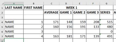
I have a very large excel sheet with 5 separate numbers for each week.  I want to have cells highlighted if they match a certain criteria and I am having issues.

Example:

If cells in column C are in the below categories, columns D, E & F would highlight if they match the second portion of the category.  This would then go on for 32 weeks with the average changing each week.

     (115 avg or less = 150-174)

     (130 avg or less = 175-199)

     (145 avg or less = 200-224)

     (160 avg or less = 225-249)

     (180 avg or less = 250-274)

     (200 avg or less = (275-289)

Any help would be wonderful.

Kim

[#2]

Under conditional formatting, you need 6 formulas (these apply to columns D through F):

=AND($B3<=115,C3>149,C3<175)

=AND($B3<=130,C3>174,C3<200)

=AND($B3<=145,C3>199,C3<225)

=AND($B3<=160,C3>224,C3<250)

=AND($B3<=180,C3>249,C3<275)

=AND($B3<=200,C3>274,C3<290)

In cases where the average changes (i.e. column H), you will need 6 new formulas for column H in order to apply to columns I through K (since the first formulas only refer to column B).

Hope this helps!

Brent.

[#3]

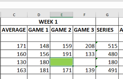
@macrordinaryI tried what you suggested but changed the $B3 to $C3 since that was the column the average was in and when it matches the formatting it highlights the cell after it.  I want the cell that contains that match to be highlighted.

Any suggestions?

[#4]

@KimKrebs For the conditional formatting (in cell C4, for example), the $C4 cell should contain the average, and the D4, E4 and F4 cells should contain the values.

So in cell E4, the conditional formatting should be:

=AND($C4<=115,E4>149,E4<175)

=AND($C4<=130,E4>174,E4<200)

=AND($C4<=145,E4>199,E4<225)

=AND($C4<=160,E4>224,E4<250)

=AND($C4<=180,E4>249,E4<275)

=AND($C4<=200,E4>274,E4<290)

Once this is done, you can copy the conditional formatting to cells D4 through G7.