Formatting Excel cells

[johnnyschiele1]

Not sure if I'm explaining this correctly, but I would like to format cells to change to RED if the value is within 500 miles of another cell.  

In the sample pic attached, if cells N2, P2, R2, or T2 are with 500 miles of J2, I'd like to have the cell either Fill red or at least change font to red.   I'm sure that it's possible, just not experienced enough to figure it out on my own.   Thanks in advance.

[#2]

That could be conditional formatting rule with formula like

=(ABS(N2-$J2)<=500)*ISEVEN(COLUMN(N2))

applied to your $N$2:$T$7 range with any format you prefer

[#3]

I'm sorry, I do not understand that formula. Again, noobie here. Don't I have to have some sort of IF/THEN?

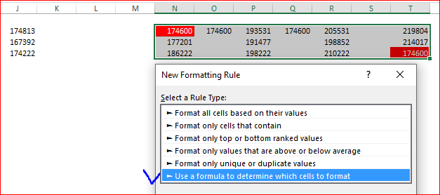
[#4 · Accepted solution]

Let me explain on your sample. First, select your range and under Conditional formatting select New rule like this

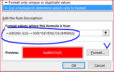
The rule is triggering applied format if the formula for it returns TRUE and ignores the formatting otherwise

First part of the formula returns TRUE if any the value of the any cell in the range is less than 500 from the value of the correspondent cell in column J

=(ABS(N2-$J2)<=500)

(please be care about absolute and relative references). But you don't need to apply format for the columns O, Q, etc. Second part of the formula returns TRUE if your cell is within every even column (N, P, etc)

=ISEVEN(COLUMN(N2))

Multiplication of both part is equivalent of AND condition, thus entire formula triggers formatting (other words returns TRUE) if both your cell is in even column and the value of the cell is differ from  the value of the correspondent cell in column J on not more than 500.

How it works is in attached file.

[#5]

Thank you so much.  I should have thought to come here sooner.  I've been driving myself nuts with this for ages.