FORMAT A CALCULATED CELL DATE RED IF THE DATE IS EARLIER THAN TODAY

[JBROCK51]

My spreadsheet has a date of last production in K3

Cell L3 is a simple formula =sum(K3+730) to show me 2 years after K3

I want cell L3 to fill with RED and change font to White Bold Italic if the calculated date in L3 is less than today.

My thought was: IF(L3<TODAY(),xxx with the x's being the part I'm not sure how to do.

Can someone help? Thank you. I'm 69 yrs old and trying to learn more complex formulas to "open my world".  I used to tell people on a scale of 1-10 I was a 7 in Excel. Now I tell them I'm a 2. Thanks in advance! - Joe

[#2 · Accepted solution]

@JBROCK51 

Hi how are you doing? I hope I can assist you

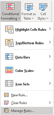
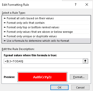
What you need is Conditional Formatting 

The formula is like the follows

=$L3<TODAY()

[#3]

@JBROCK51 

hi 

you need conditional formatting. See the attached spreadsheet where  I have inserted the formatting. 

[#4]

@Poogermum 

I completely described the wrong issue. What I in fact need to do is insert a word in Cell J3 if the calculated date is equal to or over 2 years old.  Here again is the issue, with corrected text:

My spreadsheet has a date of last production in K3

Cell L3 is a simple formula =sum(K3+730) to show me 2 years after K3

I want cell J3 to populate with the word "Partial" if the date in L3 calculates less than 2 years, or "Full" if the date in L3 is equal to or older than 2 years.  I can then use Conditional Formatting to differentiate between "Full" and "Partial".  I have attached a sample of what I'm looking for. Sorry for wasting your time the first time.

Joe

My thought was: IF(L3<TODAY(),xxx with the x's being the part I'm not sure how to do.

Can someone help? Thank you. I'm 69 yrs old and trying to learn more complex formulas to "open my world".  I used to tell people on a scale of 1-10 I was a 7 in Excel. Now I tell them I'm a 2. Thanks in advance! - Joe

[#5]

Thank you for responding. @Juliano-Petrukio