finding the everage from a column of numbers but ignoring the cells in which the value is zero

[meirtu]

Hi, How do I find the average of a column of cells, while ignoring the cells in which the value is zero? Let's say 3 out of 6 cells which are under the average formula have a zero value, then I want Excel to average only the other three cells which have a value. just to make it clear: if the column of cells under the formula are: 2, 0, 2, 0, 2, 0 - then the average result should be 2

Thanks in advance

[#2 · Accepted solution]

@meirtu 

Perhaps

=AVERAGEIF(A1:A6,"<>0")

[#3]

@Sergei BaklanThanks!! this works great!! why should there be a coma before the quotation marks in the formula?

[#4]

@meirtu , you are welcome.

It separates second parameter which defines criteria, please see here AVERAGEIF function 

[#5]

@Sergei BaklanThanks Sergei! I will definitely carefully read the tutorial link you sent me to better understand this wonderful formula, and also read about some other formulas which are not clear to me.

[#6]

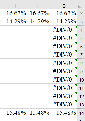
@Sergei BaklanHi again. actually checking again, this formula does not work! it does not work because in some of the percentage cells in the column there is an #DIV/0! error. This error appears because the sums in some of the cells on which the percentage has to be calculated have not been fed yet, and will only be fed as the year proceeds (it's a monthly interest percentage calculation). Is there a possibility of calculating the percentage in the percentages column without dividing? Because division will allways result in division of zero until all the cells are fed. Or maybe some other solution

Thanks in advance

[#7]

@meirtu 

You may wrap it by IFERROR returning in case of error empty text or any other value you prefer

=IFERROR(AVERAGEIF(A1:A6,"<>0"),"")

[#8]

@Sergei BaklanThanks, but for some reason it still is not working. The formula yields no result.

I am sending you the actual sheet after writing the formula as you stated. If you would be kind enough to look what is still preventing this from working, I would be so grateful. Please note that the sheet is laid from right to left, and the relevant formula is written in cell E14.

Thanks again

[#9]

@meirtu 

Sorry, I misunderstood you, though entire formula returns an error (that happens if all cells are blank).

With errors inside the range there are several ways to avoid, couple of them:

for the column G formula is

=AVERAGEIFS(G2:G13,G2:G13,"<>0",G2:G13,"<>#DIV/0!")

which ignores both zeroes and this concrete error. 

But it will be much better if you clean your data within the range, in column H formulas are

=IFERROR(IF(D2,D2/B2,""),"")

which returns empty string if any of D2 or B2 is zero. Or, as variant in column I

=IF((D2=0)+(B2=0),"",D2/B2)

With that you may use simple AVERAGE, it ignores all texts

=AVERAGE(H2:H13)

[#10]

@Sergei BaklanThanks Again! the first option you gave works wonderfully! I checked several times. I Prefer it to the second option you gave. Can I just ask about the first option why the range is repeated twice ate beginning? (G2:G13,G2:G13........)

[#11]

@meirtu , you are welcome, glad to help.

Previous time was AVERAGEIF() function, here is another one, AVERAGEIFS function 

It requires separate ranges for each criteria and another one for the average itself.  AVERAGEIF uses only one range and one criteria.

[#12]

@Sergei BaklanThanks. It's much clearer now