Finding the column name for a value in a table

[Peter Johansson]

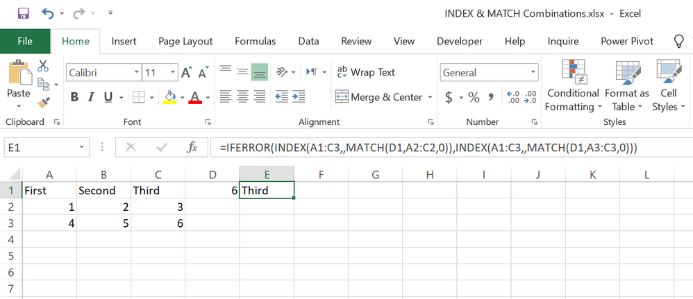
I have a 3x3 table with a header and two data rows as below.

A1=First, B1=Second, C1=Third
A2=1, B2=2, C2=3
A3=4, B3=5, C3=6

In cell D1 I'd like to enter a search criteria. For example 5.
Then in E1 I'd like to output the name of the header for that column. In this case Second.

Following the logic this should be the result in E1 when entering each number in D1.

1 = First
2 = Second
3 = Third
4 = First
5= Second
6 = Third

I've tried Index, Match and Vlookup without success. How can you solve this? :)

[#2]

Hi Peter,

You need to the Index & Match combination to solve this!

But you need to nest another combination because you want to search the value in cell E1 in two rows!

The formula looks like this:

=IFERROR(INDEX(A1:C3,,MATCH(D1,A2:C2,0)),INDEX(A1:C3,,MATCH(D1,A3:C3,0)))

 

Hope that helps

[#3]

That helps, thanks :)

What if I want to expand the table with more columns and rows? Is it possible to make the formula more dynamic?

[#4 · Accepted solution]

Idea is here https://exceljet.net/formula/get-location-of-value-in-2d-array

[#5]

Thanks,

That works like a charm :) Let's say these numbers were part of a zip code.

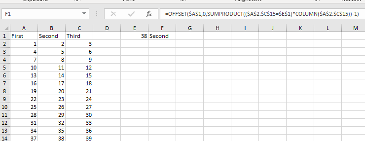
So in E1 I would enter 38000. Instead of the part: $A$2:$C$15=$E$1
I'd like: $A$2:$C$15=LEFT($E$1;2)

But I get a #REF! error. What can be wrong in this case?

[#6]

Peter, LEFT returns text, wrap it with VALUE to receive number

=OFFSET($A$1,0,SUMPRODUCT(($A$2:$C$15=VALUE(LEFT($E$2,2)))*COLUMN($A$2:$C$15))-1)

[#7]

Works great. Thanks again :)

[#8]

You are welcome

[#9]

please help me out, i need a formula to select coloumn name, on basis of finding the min value .

i need a formula to selection-1 and selction-2 for selecting vendor with min values

place	vendor-1	vendor-2	vendor-3	vendor-4	selection-1	selection-2
USA	5000	7000	5000	8000	vendor-1	vendor-3
INdia	9000	8000	8000	9500	vendor-2	vendor-3

[#10]

@Sergei Baklan 

IF value is in one or more than cells than i want to show all the column name that have value

[#11]

@AZUBHAN 

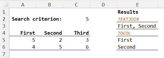
If you want the result as a comma separated list you could use

= TEXTJOIN(", ",,IF(data = searchCriterion, header, ""))

To obtain a list 

= TOCOL(IF(data = searchCriterion, header, NA()),3)

Each formula tests every cell of the data table and uses a function to filter the results.

[#12]

The problem we have here is that we are assuming that there will be no repeat values. As soon as there are then the column numbers will be added which gives the wrong result. Enter "38" into A7 for example and you will return Third (1+2).

[#13]

@John_Bainbridge 

Too old thread...

Yes, you are right, it is assumed we have unique values. For the modern Excel @Peter Bartholomew gave the solution above. For the legacy Excel to return first column where the value appears it could be like

=IFERROR(
    INDEX(
        $A$1:$C$1,
        AGGREGATE(
            15,
            6,
            1 / ($A$2:$C$15 = $E$1) * COLUMN($A$2:$C$15),
            1
        )
    ),
    "no such"
)

To show few columns with the target value it could be

=IFERROR(
    INDEX(
        $A$1:$C$1,
        AGGREGATE(
            15,
            6,
            1 / ($A$2:$C$15 = $E$1) * COLUMN($A$2:$C$15),
            COLUMN()-COLUMN($J$1)+1
        )
    ),
    ""
)

and drag it to the right till first empty cell appear.