Finding bottom 10 values with criteria

[willc8]

Hi all,

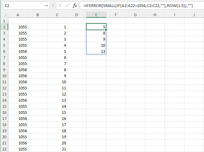
I'm currently currently trying to pull the bottom 5 values from a table based off of criteria. The criteria is a ID # ex. "1056" and the other data I want to rank is distance. To do this I found this.

=small(IF(A2:A20="Value",C2:C20,""),ROW(A1:A10))

I've tried to use it but it just won't work returning the #NUM! error every time. Based off what I could find online I've narrowed it down to some sort of formatting issue but no matter how I try to format my data it wont work. Does anyone have any advice?

[#2]

@willc8 

Are your IDs numbers or text? If they are numbers, omit the quotes around the value:

=IFERROR(SMALL(IF(A2:A20=1056,C2:C20,""),ROW(1:5)),"")