Find Trimmed Mean of all the values of an item

[Kenechukwu_Oraelosi]

Update: Thank you for the correction. Thing is i'm new to VBA and have no idea even how to begin to write the code required. I will try to explain my desired goal in the details below. This is for a personal project and i just got introduced to excel to try to pull it off so i have no idea how to start and put it all together. I use Excel 2013

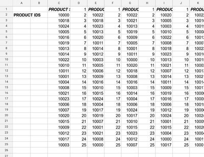
On the Analysis2 sheet, Each 'contractes' column is a list of of product IDs. There are 25 product IDs in total. The numbered row beside each list of product IDs are the ratings for the top 20 products from the set of products by the customers in each survey. There were 20 sets of product ID and rank columns for 20 surveys in all

What i would like is a VBA scrip that would rank products by their average quality rating

Data sheet (starting point):

In the sample sheet i've gone through the process manually to show the expected result at each stage, but if you notice there are no formulas or macro attached to the workbook. What i would like is a vba script that achieves the same process. I believe it needs to be a vba script because i believe it would have to loop through each column of data performing a set of actions, before moving on to the next column

The analysis2 sheet is generated from filtering and then merging the survey results from their individual sheets into a single sheet. There will be new product surveys performed so the range in analysis2 sheet is dynamic and would expand over time so the vba script would need to work on a dynamic range

Here are the steps:
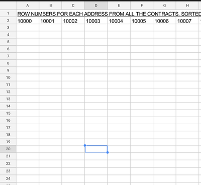
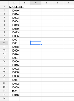
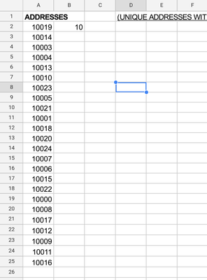
I would like to first generate both a row of the unique list of the product IDs in sheet3 and a column of the unique list, in report sheet, both from the analysis2 sheet

 

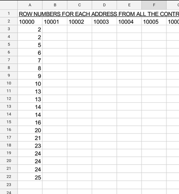
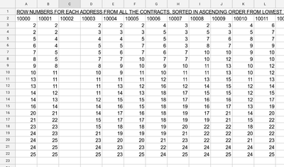
Then i'd like that For each product ID in sheet 3, it would index its value in analysis2 sheet, find its rank in the adjacent column, list it in a column under its ID in sheet 3. and repeat that through the range until it has listed all its rank numbers in a column.

Then go to the next product ID in sheet3, and repeat the same process till it has listed out all the ranks for all the product IDs

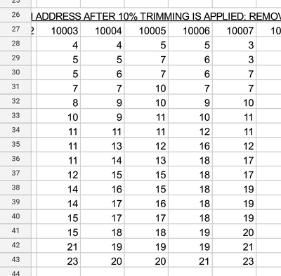
Once it has done this, it would then sort each column in sheet3 from least to most

 

After sorting, it would then go through a product ID column in sheet3 and find the trimmean of the rank numbers. Using for example a 10% trimming, this would mean removing the top 10% and bottom 10% of values, in this case the top 2 and bottom 2 rank numbers, and then finding the mean of the remaining 16 rank numbers. This is done to remove some effect of outliers.

It would then go to the product ID in report sheet and paste the trimmean in the adjacent column. It would then repeat this for the next product ID column until it completes all the product IDs.

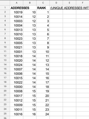
Finally it would then sort the column of product IDs in report sheet by the trimmean values in the adjacent column, from least to most. This would give the product IDs that are on average ranked highest to Lowest in all the surveys by customers. It would then generate a column of row numbers in an adjacent column to show their ranks

 

Again, my apologies for taking this long to respond. I am totally stumped on how to proceed on this and would appreciate all help

I am still new to forums and haven't fully understood the rules, including the one on cross posting. Below are all the other forums this question has been posted in:

1. https://www.excelforum.com/excel-programming-vba-macros/1391443-find-trimmed-mean-of-all-the-values-...
2. https://forums.excelguru.ca/threads/find-trimmed-mean-of-all-the-values-of-an-item.11623/
3. https://techcommunity.microsoft.com/t5/excel/find-trimmed-mean-of-all-the-values-of-an-item/m-p/3655...
4. https://www.mrexcel.com/board/threads/find-trimmed-mean-of-all-the-values-of-an-item.1219566/
5. 
6. https://stackoverflow.com/questions/74104762/find-trimmed-mean-of-all-the-values-of-an-item

[#2]

You've had 70 views as of this writing, but no replies. I suspect that's because it's not entirely clear what you're asking help in accomplishing. When I look at your spreadsheet, it appears as if you have most of it already done. You also make a point of wanting a visual basic routine, when it's not at all clear why THAT needs to be involved. So I wonder if you could take a few minutes to spell out more fully what it is that you're seeking; the work you've already done shows a fair amount of familiarity with Excel, making me at any rate wonder what I'm missing.

[For the record, if it makes a difference, I personally prefer to avoid VBA and macros, choosing instead to figure out ways that Excel's many functions can achieve the results. There are plenty of other folks here in this forum, however, who are adept at VBA if that indeed is a "must"]

[#3]

Sorry i took time. I updated the original post explaining in detail what i need and why i think it needs to be macro. Also the sample sheet i uploaded was done manually - no VBA code or formula (mostly). What i would like is a VBA script that does the same thing automatically

[#4]

@Kenechukwu_Oraelosi 

I did a PQ solution with the TRIMMEAN function provided by Imke Feldmann.