Filter no choice between number and text

[skylanetk]

In a table when I put in a filter and I want a number filter EXCEL automatically puts in a text filter and I want a number filter. EXCEL Does not give me a choice. There are blank cells in the column because I have written logic to return a number or,"",. I know that EXCEL recognizes the ,"", as text. I know that if I put in 0s it will give me a number filter but then if I want averages they will be wrong because of adding 0s so I then get a number filter. WHY doesn't EXCEL allow me to make the choice? Is there another way to do it?

[#2]

@skylanetk 

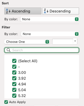
I can't answer the question why it doesn't give you a choice, because when I went and looked for an example in one of my own spreadsheets, it DID give me a choice. The formula that I have for that column  has exactly the same logic as yours, returning either "" or a number. And this image shows what I get in the Dialog box if I ask to filter. 

So could you give a more detailed picture (literally or figuratively) of what happens in your situation?

[#3]

It is my understanding the if more numbers show up in the column then ,"", text responses EXCEL automatically makes the number filter show. The problem comes if the "" text response is the larger then EXCEL automatically chooses the text filter and you don't have a choice. Then you must make your answer in all of the cells in the column numeric. That creates other problems when you say average the numbers in the column.

[#4]

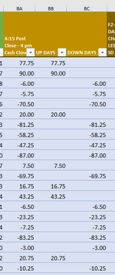
Above is my example, Column BA shows the daily  price changes of the index.  Then I used these formulas to separate the up days and the down days into their own columns.

Up days: =IF($BA2>=0,$BA2,"")

Down Days: =IF($BA2<0,$BA2,"")

So column BB gives me a number filter and I can then filter for different values.

Column BC only gives me a Text Filter and no choice to make it a number filter. The only way I can use it to filter different number values is to make more columns getting those values out of the column or making the entire column numeric.

[#5]

You could change your formula to return a "0", and then us an averageIF formula that ignore's zeros.

Not sure if there are other zero's in your data though.

[#6]

@skylanetk You wrote:

It is my understanding the if more numbers show up in the column then ,"", text responses EXCEL automatically makes the number filter show. The problem comes if the "" text response is the larger then EXCEL automatically chooses the text filter and you don't have a choice. Then you must make your answer in all of the cells in the column numeric. That creates other problems when you say average the numbers in the column.

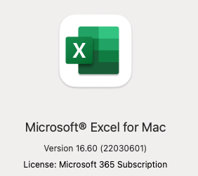
But my column--the one from which my image of the filter dialog box was taken--has more cells with the "" value than with a numeric value. Yet it's still showing as it is pictured.  It's possible we're working with different versions of Excel, I suppose. Mine is the most recent version.

[#7]

It should not be so difficult it should be my choice. And adding a 0 also means I will have to add more steps in other places. There are also other advantages to seeing empty cells.

[#8]

I am a Microsoft office user also, Microsoft 365.

[#9]

@skylanetk 

Looking more closely at your image, it appears that we're both working with stock market data. And looking at your two adjacent columns, I have a suggestion:

Why don't you use conditional formatting to differentiate the Up days from the Down? All of the Downs are negative values, the Ups are positive. Excel can automatically show negative numbers in red, positive in black. Put them all into one column which would then be all numeric.

[#10]

because I am not only interested in the fact that a day is negative or positive , I need to know the size of the changes. It is only one factor out of hundreds that I look at.

[#11]

@skylanetk 

Of course you're interested in size, i.e., magnitude of numbers, not just direction (positive or negative), and that's why what I wrote mentioned Excel will automatically highlight negative NUMBERS in red, positive in black.

I do the same. I also use FILTER and other functions to extract those with largest magnitude (positive or negative) or largest change.....

My main point was to say if you're trying to use the Filter menu tool and running into obstacles because of the numeric vs text matter that you posted about, there are other ways to accomplish your objective. Excel almost always offers users different routes from point A to point B...part of the fun of using it is to explore those alternative routes. 

[#12]

@mathetes 

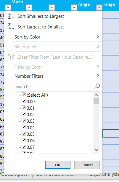
This is what I am talking about. Sometimes I want a number filter and I do not get a choice. thank you for your response.

[#13]

@skylanetk 

That's a very different Filter dialog box than the one I see. What version of Excel are you using? Mine is the most current version.

Do you have access to the FILTER function? A new "Dynamic Array" function...it also requires the most current version of Excel....given the kind of thing you're doing, I think you'd find it worth your while to have it.

https://www.youtube.com/watch?v=9I9DtFOVPIg

[#14]

@skylanetk So what I have had to do sometimes is change the query setting. For whatever reason sometimes the Columns will be set as Text type. If this is the case then when you query the data into your Excel spreadsheet go to the Query Tools tab on the toolbar.

1. Click Edit

2. The Power Query Editor should pop up

3. Select the columns you need to change to Number type

4. Under the Transform section on the toolbar there is a dropdown for Data Type

5. Select the type you need

[#15]

You could add conditional formatting to the column to highlight blank cells, then filter by color; or create a second column next to the column where you want to continue to see empty cells that adds a 0 so you can use the secondary column to use a number filter. Otherwise, you'll have to live by Excel's limitations.

[#16]

@xsmplfy Thank you for the reply. Good options, I just want it to be an easy choice. I do quantitative

analysis on the markets. I look at hundreds of variables in every decision model, so doing it a few times would be alright but some of my data models have a thousand columns of data before I even start any analysis. So now for the most part I tabulate data, move it and do analysis in other tables.