Fill background color of cell 1 if cell 1 is included in cell 2 formula

[bapatri]

I am trying to add a fill color to cell 1 if cell 1 is included in the formula of a cell 2.

Also, it would need to remove fill color from cell 1 if it is removed from cell 2.

I have attached an example.

Is this doable?

[#2]

@bapatri 

I'm confused when you say "included in the formula ..." you mean the value as a result of the formula or the range (AC75) on the formula itself?

[#3]

@Juliano-Petrukio The range of the formula. 

[#4 · Accepted solution]

@bapatri 

I need to admit that it is the first time I see something like that.

Well, the conditional formatting formula would be something like that.

=FIND(SUBSTITUTE(ADDRESS(ROW(),COLUMN()),"$",""),FORMULATEXT($B15))>0

 Remember to change the reference where the "main" formula is. This case the formula is on B15

Find attachment.

[#5]

@Juliano-Petrukio 

This should work!
AND I admit I am not very fluent with excel.
I have attached the file in question.

Ideally, I would be able to assign a color to the total from the high, medium and low priority cells, and excel would magically fill in the background colors of all cells included in the range of the formula.

[#6]

@bapatri 

[#7]

It works, thank you!!
I can't figure out how to duplicate to other cells. Any advice or tutorials?

[#8]

@bapatri 

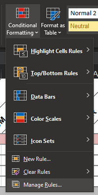
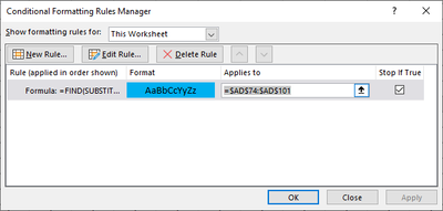
You just need to select the cells you want to apply the formatting

On Applies to you change the range you want to apply

[#9]

Perfect, thank you.

[#10]

Anytime.
Remember that hitting the like button is less costly than buying me a coffee.

[#11]

@Juliano-Petrukio 

I did virtually the same as you, with the exception that I used a column of defined names to identify the references rather than using ADDRESS and direct referencing.  My feeling, though, was to write,

"yes, what the OP requires is technically possible using FORMULATEXT, but I wouldn't recommend it". 

I would prefer to see a specific data field to hold the {"high","medium","low"} and drive the formula from the data rather than the reverse.  What are your thoughts?

[#12]

I agree with you but sometimes the user wants something like that.
For sure with time we can propose a simpler solution and I hope more topics can be raised by him very soon with more challenges.
As I told "(...) it is the first time I've seen something like that." It was fun to assist him somehow.

[#13]

@Juliano-Petrukio 

Just to 'come up with the goods' and demonstrate that I had come up with a similar solution.

Mine probably has higher set up costs because I used defined names, but, then, I use defined names for everything.