extract player names following text string references

[steveccc]

Hello, I have converted a csv file into an Excel workbook. I would like to extract player names between specific text strings.

The data is in column B. I would like to extract the player names in columns C:J. 
Column headers are in row 1.

For example, the data in Cell B2 is:

F Brandon Ingram G Ja Morant PF LaMarcus Aldridge SG Lou Williams PG Kemba Walker UTIL Draymond Green SF Danuel House Jr. C Bismack Biyombo.

Column Headers B:J are: PG SG SF PF C G F UTIL

I would like cells B2:J2 to contain the full player names under their proper column headers like this:

Cell H2: Kemba Walker, Cell I2: Lou Williams, Cell J2: Daniel House Jr.,

I made an attempt with a "mid find" formula, but it really does not work well (see attached).

Some names are composed of 2 words or 3 words, so this may make it a little tricker. Also, Some player names start with G, and this causes the formula to retrieve the wrong player name (see cell H2 for example. Cell H2 should contain the name "Lou Williams").

Thanks so much for the help and Happy Thanksgiving!

[#2]

Hello,

It will be good to use Text To Column to split all the data by the Space delimiter (see the same excel file with the solution attached)

1. Select all from B2 downward using CTRL + SHIFT + Down Arrow.
2. Click on Text To Column in the Data tab
3. Click on Next.
4. In the Step 2 of 3 wizard dialogue box, uncheck Tab and check Space
5. Click Next
6. Optionally, you cab choose Cell Destination.
7. Click Finish

Then, use CONCATENATE or CONCAT function to join First and Last Name.

That's what I did in the solution attached. Kindly let me know if this helps...

Regards,

[#3 · Accepted solution]

@steveccc 

Variant with Power Query is based on idea here https://bondarenkoivan.wordpress.com/2015/04/16/multiple-replacements-of-words-in-power-query/

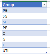
First, we create table with separators 

and with query add column to which transform separators, like "PG " => "* PG "

With above function we transform source table into

and split column into rows by "* " delimiter

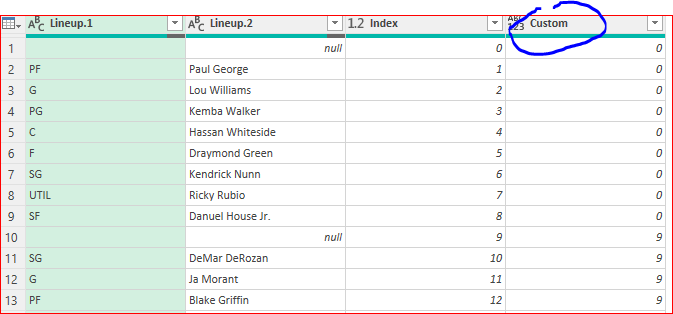
adding index and conditional column we give unique number to each group of names

Filter nulls, remove Index and pivot Lineup.1 on Lineup.2 with rows aggregation. Remove Custom column and load result back to Excel sheet.

That is in the second sheet of the attached file.

If source data is in csv file you may connect it directly instead of data table as here.

[#4]

Thanks very much for your time Abiola1. Your solution would work, but I'd like to use a less labor intensive process that uses functions and formulas if possible. I feel like I'm half way there using something close to this: =TRIM(MID($G2,FIND(H$1,$G2)+3,10))

[#5]

Sergei Baklan thanks for these instructions. I haven't used Power Query before, so this will be a big help for me in general. Ultimately I would like to get a solution that uses functions/formulas though.

[#6]

@steveccc 

If with formula I'd suggest first to wrap headers with spaces, i.e. use " PG " instead of "PG", and the formula

=IFERROR(MID($B2,
   IF(RIGHT(D$1,LEN(D$1)-1)=LEFT($B2,LEN(D$1)-1),
      0,
      SEARCH(D$1,$B2)
   ) +
      LEN(D$1),
      IFERROR(
         AGGREGATE(15,6,
            1/(IFERROR(SEARCH($D$1:$K$1,$B2),1)> IF(RIGHT(D$1,LEN(D$1)-1)=LEFT($B2,LEN(D$1)-1), 1,  SEARCH(D$1,$B2)))*
            IFERROR(SEARCH($D$1:$K$1,$B2),1),1
         ),
      LEN($B2)
      ) -
      IF(RIGHT(D$1,LEN(D$1)-1)=LEFT($B2,LEN(D$1)-1),
         1,
         SEARCH(D$1,$B2)
      ) -
      LEN(D$1)
),"")

in D2, drag it to the right and all down.

Please check third sheet in attached file.

[#7]

@Sergei Baklan Wow this is amazing. Thanks Sergei Baklan!

One small thing, I noticed some players are missing the last letter of their name.

For example, Cell K13 is missing a "k" -- "Russell Westbroo", should instead be "Russell Westbrook".

Cell G7 is missing an "e" -- "Paul Georg" should instead be "Paul George".  Cell K15, K20, H23, H24, and a few others...

I tried modifying the code but it didn't work for me.

[#8]

@steveccc 

I see, sorry for the bug. I'll try to correct bit later.

[#9]

@steveccc 

That was for the first and last elements in the text. I corrected initial formula (4th sheet attached) and simplified it a bit

=IFERROR(MID($B2,
   SEARCH(D$1," " & $B2)-1 + LEN(D$1),
      IFERROR(
         AGGREGATE(15,6,
            1/(SEARCH($D$1:$K$1," " & $B2)> SEARCH(D$1," " & $B2))*
            SEARCH($D$1:$K$1," " & $B2),1
         ),
      LEN($B2)+1
      ) -
      SEARCH(D$1," " & $B2) - LEN(D$1)+1
),"")

in a 5th sheet attached. Please check if it works.

[#10]

@Sergei Baklan This is perfect. It is a work of art. Thank you so much!

[#11]

@steveccc , you are welcome, glad to help

[#12]

@Sergei Baklan 

Hello Sergei, I'm trying to follow your Power Query instructions above. I'm new to Power Query, so none of it is intuitive. Are you able to post more detailed instructions? I searched a few videos on YouTube and could not find anything directly relevant, so I thought I could ask you. If you have a YouTube channel, please let me know. Here is what I figured out on my own.

Step 1: 
Source data is in B1:B151.
In Excel worksheet, create a table of separators in D1:D10.

Step 2:
Highlight source data B1:B151.
Goto Data drop down menu.
Select "From Range / Table"
This opens up Power Query.

Step 3: 
Sadly, this is where I am stuck. 
How do I do this?
"and with query add column to which transform separators, like "PG " => "* PG "

If you have time, I'd love to get step by step instructions because I'm brand new to Power Query. Thanks for considering this!

[#13]

@steveccc 

I will update with step by step instruction bit later.

As for recommended source - not sure, it's a lot of information in internet. You may start from Excel template. File->New and search for it as

[#14]

Thanks again.

[#15]

@steveccc 

One question - do you copy/paste or insert source data (B1:B151) from csv file? If so it'll be easier to query it, i could update the query if you give a sample of such file.