Extract list with only allowing duplicates if item is shared

[choongko]

Hope someone can help me with a solution to extract the list (TaskID) assigned to the groups.  The TaskID should only duplicate if they are assigned to more than one group.    This part was the issue I am facing.  Thanks. 

[#2]

@choongko 

I'd create a pivot table - see the attached version.

[#3]

@choongko 

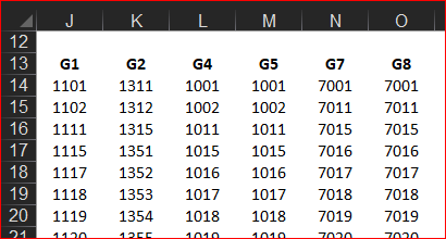
As variant with formulae

J13:

=TRANSPOSE( UNIQUE( SampleData[Grp] ) )

J14:

=SORT( UNIQUE( FILTER( SampleData[[Task ID]:[Task ID]], SampleData[[Grp]:[Grp]]=J13 ) ))

and drag to the right

[#4]

@choongko 

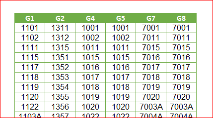
One more variant is with Power Query

Script is

let
    Source = Excel.CurrentWorkbook(){[Name="SampleData"]}[Content],
    #"Remove Unused" = Table.SelectColumns(Source,{"Grp", "Task ID"}),
    #"Added Index" = Table.AddIndexColumn(#"Remove Unused", "Index", 0, 1, Int64.Type),
    #"Removed Duplicates" = Table.Distinct(#"Added Index", {"Grp", "Task ID"}),
    #"Remove Index" = Table.RemoveColumns(#"Removed Duplicates",{"Index"}),
    #"Grouped Rows" = Table.Group(
        #"Remove Index", {"Grp"},
        {{"Tasks", each List.Sort(_[Task ID] ) }}
    ),
    ToTable = Table.FromColumns(#"Grouped Rows"[Tasks], #"Grouped Rows"[Grp])
in
    ToTable

[#5]

Tks for the reply. Is there anyway to use formula for Excel 2016? I tried not to use pivot table if possible.

[#6]

@choongko 

Advanced Filter would be another solution, but here is one using formulas:

[#7 · Accepted solution]

@choongko 

That could be

J59:

=IFERROR( INDEX(
  SampleData[[Grp]:[Grp]],
 AGGREGATE(15, 6,
      1/(COUNTIF( $I$59:I59,  SampleData[[Grp]:[Grp]] )=0)*
     ( ROW( SampleData[[Grp]:[Grp]] ) -
       ROW(SampleData[[#Headers],[Grp]] ) ),
  1)
 ), "")

drag to the right till empty cells appear

J60:

=IFERROR( INDEX( SampleData[[Task ID]:[Task ID]],
     AGGREGATE(15, 6,
       1/
         ( SampleData[[Grp]:[Grp]] = J$59 ) /
         ( COUNTIF(J$59:J59, SampleData[[Task ID]:[Task ID]] ) = 0)*
     ( ROW(SampleData[[Grp]:[Grp]] ) -ROW(SampleData[[#Headers],[Grp]]) ),
      1 ) ),
 "")

drag to the right and entire line down.

[#8]

Tks for the solutions. Appreciate it. Solved.

[#9]

Thanks Hans, Appreciate it. It works too...

[#10]

@choongko , you are welcome, glad to help