Excel Start & Finish Time with with Operating Hrs each day

[Jeev125]

Hi All,

Need a solution for the below. i have start and finish time but it expands to approx 8-9 days. how do i calculate total hrs with only operating hrs which starts from 4:20 am and finish at next day 1 or 2 am. 

In below example i need actual value as my end result cant go with total which includes non operating hrs.

Start	Finish	Total			Operating HRs
15-06-2020 11:59:05 AM	23-06-2020 09:06:05 AM	189:07:00			Sunday	4:20	1:00
					Monday	4:20	1:00
		Actual			Tuesday	9:06	1:00
		~176hrs			Wednesday	4:20	1:00
					Thursday	4:20	1:00
					Friday	4:20	2:40
					Saturday	4:20	2:40

[#2]

@Jeev125 I would say you take the total and subtract the #day * the down time but saying 1 or 2 am makes it impossible to know unless there is a complete list of hours each day or something.  Furthermore your example doesn't follow your criteria. If there were 8 days and you are shutdown for at least 2am - 4:20am that is >2hrs a day or more than 16hours over 8 days which means the actual hours has to be LESS than 173 hrs and really a max of about 170 hrs but your "actual total" of ~176 hrs is MORE than that which doesn't make sense with the other data/info you gave.  We, or at least I, need more clarification.

[#3]

Hi @mtarler 

If i take difference between start & finish time which is around ~189 as stated in table (Total), but if exclude non operating hrs from start to finish to be exact i get.

176:54:50

i get the actual value when i do calc for each day and sum. 

what i am trying to achieve to get formula in single cell to dictate the working hrs only in compliance with Operating Hrs fro each day.

[#4]

@Jeev125 

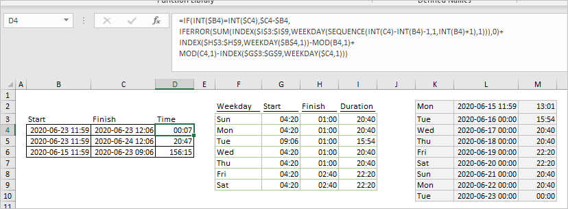
Perhaps like this

if I understood the logic correctly (can't receive 175 manually as in the grey range).

In shifts range Finish is the time on next day, i.e. =25/24 fo Sun, etc. Duration=Finish-Start.

Formula for operating time

=SUM(INDEX($I$3:$I$9,WEEKDAY(SEQUENCE(INT(C4)-INT(B4)-1,1,INT(B4)+1),1)))+
INDEX($H$3:$H$9,WEEKDAY($B$4,1))-MOD(B4,1)+
MOD(C4,1)-INDEX($G$3:$G$9,WEEKDAY($C$4,1))

assuming your version of Excel supports dynamic arrays.

[#5]

@Sergei Baklan 

Your Formula works only if there is more 2 day difference if its one day then it shows Clac Error and if its sameday then it shows Value Error.

Could you please help me with the issue.

[#6]

@Jeev125 

Please check the update, formula is

=IF(INT($B4)=INT($C4),$C4-$B4,
IFERROR(SUM(INDEX($I$3:$I$9,WEEKDAY(SEQUENCE(INT(C4)-INT(B4)-1,1,INT(B4)+1),1))),0)+
INDEX($H$3:$H$9,WEEKDAY($B$4,1))-MOD(B4,1)+
MOD(C4,1)-INDEX($G$3:$G$9,WEEKDAY($C4,1)))

[#7]

@Sergei Baklan 

You are genius, but i found a small flaw, I have attach the attachment for you. Please let me know.

[#8]

@Jeev125 

Sorry, forgot about overnight shifts. Will play with that bit later.