- Subscribe to RSS Feed
- Mark Discussion as New
- Mark Discussion as Read
- Pin this Discussion for Current User
- Bookmark
- Subscribe
- Printer Friendly Page
- Mark as New
- Bookmark
- Subscribe
- Mute
- Subscribe to RSS Feed
- Permalink
- Report Inappropriate Content
Mar 11 2023 01:55 PM
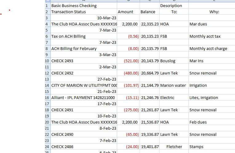
In Win 11 using Excel 2007 ( but changing over to Excel 2021 soon). How can I easily move a date row to a column to the left of the line (below the date as presently formatted) with which it is associated for a table that is over in excess of 500 rows?
- Labels:
-
Formulas and Functions
- Mark as New
- Bookmark
- Subscribe
- Mute
- Subscribe to RSS Feed
- Permalink
- Report Inappropriate Content
Mar 11 2023 10:47 PM
Solution@mikesuefle If this is a on-time task, I would do it manually. It takes less than a minute to achieve. I've assumed that the data is organised for all 500 row as your picture show. I.e. a date then one row, then a date and again one row etc.
1) Insert a column to the left of the data. Thus, everything shifts one column to the right and an empty column A appears.
2) In A2 enter the word Date
3) In A4 enter the formula =B3 and copy it all the way down.
4) Select entire column A, Copy and paste values onto itself
5) Put filter buttons on row 2
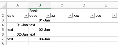
At this stage you should have something like this:
6) Press the filter button in B2 and select only the dates.
7) Select all visible rows with dates and delete the rows
8) Clear the filter from B2
The end result should be like this:
Once you have upgraded to a newer version and if this is going to be recurring task you may want to look into Power Query to automate this kind of transformation. Alternatively you could record/write some VBA code to do this, but VBA is not my kind of thing.
- Mark as New
- Bookmark
- Subscribe
- Mute
- Subscribe to RSS Feed
- Permalink
- Report Inappropriate Content
Mar 12 2023 07:36 AM
- Mark as New
- Bookmark
- Subscribe
- Mute
- Subscribe to RSS Feed
- Permalink
- Report Inappropriate Content
Mar 12 2023 08:34 AM - edited Mar 12 2023 09:07 AM
Yep, worked like a charm. Thanks again. For add'l entries will drag and drop dates to column until I change to Excel 2021.
Accepted Solutions
- Mark as New
- Bookmark
- Subscribe
- Mute
- Subscribe to RSS Feed
- Permalink
- Report Inappropriate Content
Mar 11 2023 10:47 PM
Solution@mikesuefle If this is a on-time task, I would do it manually. It takes less than a minute to achieve. I've assumed that the data is organised for all 500 row as your picture show. I.e. a date then one row, then a date and again one row etc.
1) Insert a column to the left of the data. Thus, everything shifts one column to the right and an empty column A appears.
2) In A2 enter the word Date
3) In A4 enter the formula =B3 and copy it all the way down.
4) Select entire column A, Copy and paste values onto itself
5) Put filter buttons on row 2
At this stage you should have something like this:
6) Press the filter button in B2 and select only the dates.
7) Select all visible rows with dates and delete the rows
8) Clear the filter from B2
The end result should be like this:
Once you have upgraded to a newer version and if this is going to be recurring task you may want to look into Power Query to automate this kind of transformation. Alternatively you could record/write some VBA code to do this, but VBA is not my kind of thing.


