Excel Pivot Table - Power Pivot - Average Help

[MrBuchanan]

This is my sample table data, and my pivot table. I am trying to get the pivot table to show the average duration it took for the two applications to get approved, 75.5 days. I created a pivot table with data model, and put add on for power pivot. I tried some measures, but could not get any to work, I always get 53.25, any help would be appreciated, thank you.

[#2]

Hi. I can see where the issue is occurring. Your Pivot is averaging the two entries in the PivotTable rather than the four entries in the Sample Data. Unfortunately, I can't seem to get a work around. Perhaps you need to add all the ApprovalDuration to the PivotTable and group them before averaging?

[#3]

A rather clunky work around is to include the Node ID field beneath the Power Source ID field in your Pivot Table and then collapse it. You can then average the ApprovalDuration field.

[#4]

Rather bizarrely, I've just removed the Node ID field from the PivotTable Fields List and the Average function works perfectly! Even after refreshing or adding more data, it works.

[#5]

Hi @MrBuchanan 

EDITED: Please look @Riny_van_Eekelen reply below

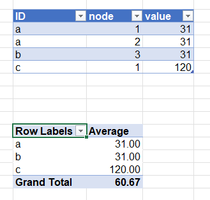
[#6 · Accepted solution]

@L z. But what if another ID also has a duration of 31 days? Then the average should become (31+31+120)/3 = 60,67

You'll need a measure that takes distinct ID's into account. Not just distinct duration values. Such a measure would look like this:

=AVERAGEX(DISTINCT(SELECTCOLUMNS('Table', "ID", 'Table'[ID], "value", 'Table'[value])), [value])

[#7]

Hello @Riny_van_Eekelen 

I realized that after posting and was going to look at fixing my bad => Thanks for doing it

(no idea why but it seems I can't delete a post here, will revise it...)

[#8]

Thank you so much, I got it to work. Now I need to study every part of it to understand it, I will do that this weekend! :)

[#9]

@MrBuchanan 

Glad I could help.

DISTINCT(SELECTCOLUMNS(----) creates a two column intermediate table without duplicate rows (ID and value). Like this:

ID, value

a, 31

b ,31

c, 120

And then the AVERAGEX function takes that intermediate table and averages the [value] column.

[#10]

Thank you for explaining.

[#11]

Hello @Riny_van_Eekelen 

I added to the measure to also include Request Power column incase two power applications are submitted 1 year apart with the same power source ID, so each average is counted, and it works good in the test file.

I did have one more question, I tried to get the measure to work in my live data tracker, and the measure returned some type of error about strings, like data cannot be a string. Is there anyway to add some type of code so it ignores these strings/invalid data when computing the intermediate table so it does not error? Thanks

=AVERAGEX(DISTINCT(SELECTCOLUMNS('MasterTracker', "Power Source ID", 'MasterTracker'[Power Source ID], "Request Power", 'MasterTracker'[Request Power], "ApprovalDuration", 'MasterTracker'[ApprovalDuration])), [Average of ApprovalDuration])

[#12]

@Riny_van_EekelenSpecifically this is the problem I am having, if the duration formula does not find a number in Power Design Received, it returns a string "", and this makes AverageX break.

[#13]

It looks like ChatGPT was able to offer a solution (I had to ask it like 8-9 times it gave me a bunch of wrong answers). Here is the solution that worked:

To fix the error caused by string values in the ApprovalDuration column, you can modify your measure formula to exclude them. Here's an updated formula that should work:

Average Approval Duration = AVERAGEX(
    FILTER(
        DISTINCT(
            SELECTCOLUMNS(
                'MasterTracker', 
                "Power Source ID", 'MasterTracker'[Power Source ID], 
                "Request Power", 'MasterTracker'[Request Power], 
                "ApprovalDuration", 
                    IFERROR(VALUE('MasterTracker'[ApprovalDuration]), BLANK())
            )
        ),
        NOT(ISBLANK([ApprovalDuration]))
    ),
    [ApprovalDuration]
)

This formula converts the ApprovalDuration column to a numerical value using the VALUE function and replaces any string values with a blank. Then it uses the FILTER function to remove any blank values and the NOT(ISBLANK([ApprovalDuration])) condition to exclude any remaining string values. Finally, it calculates the average of the numerical values using the AVERAGEX function.