Excel IF AND using range for criteria

[Jn12345]

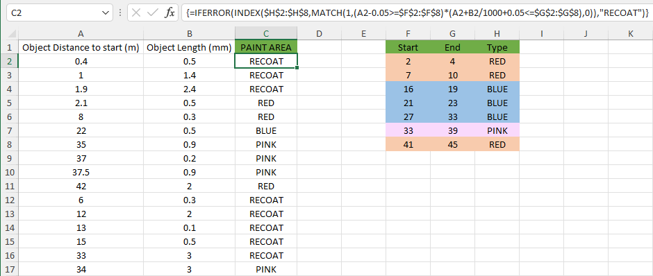
Hello, I’m wondering if I can use a formula like this =IF(AND(Value1>any value in a range of cells,Value1<any values in another range of cells) I get the whole IF(AND(range of cells>value 1) but I’m trying to do it the other way where I have a value and need to see if it falls between any row in column a (start distance) and column b (end distance) column a and b might have many rows and the table im working with only has a few rows so it’s not like I can just drag a formula beside each one. An example would be if a field is covered from say 10m to 20m and again from 25m to 30m and possible a bunch more areas going from one end to another I need to find out if in my table the objects at a certain start distance and end distance fall between any of the areas that are covered on the field. Any help will be greatly appreciated!!!

[#2]

@Jn12345 

You need OR here:

=IF(OR((value1>=start_distance)*(value1<=end_distance)), value_if_true, value_if_false)

[#3]

@Hans Vogelaar Thanks for the reply

=IF(OR(AND((A2-0.05)>$E$2,(A2+(B2/1000)+0.05)<$F$2),AND((A2-0.05)>$E$3,(A2+(B2/1000)+0.05)<$F$3),AND((A2-0.05)>$E$4,(A2+(B2/1000)+0.05)<$F$4)),"RED","NO PAINT")

Columns A is the start of the object on the field, Column B is the length of the object and E is the start of the RED paint and F is the end of the red paint. Hopefully this helps since i cant upload a photo. So Technically it isnt paint on a field but its a fairly simple analogy to make it all make sense without having to get to crazy with explanations. so, i have made the first part of the formula and there will be nested IF( functions so that i can add more options to what is returned. I will need AND in the formula since there are two criteria that must be followed in order to return a specific response. To make it a bit more complicated the Object from the first two columns has to be within the painted sections by at least 0.05m to be considered within those areas. Im trying to simplify the formula to take the entire array / table within columns E and F into the formula so that i dont have to use OR a zillion times for each row within columns E and F (and additionally for each row within H, I, K and L columns in the future). Hopefully you can understand what im trying to do from this screen shot.

[#4]

@Jn12345 

Could you attach a sample workbook (without sensitive data), or if that is not possible, make it available through OneDrive, Google Drive, Dropbox or similar? Alternatively, you can attach it to a private message to me. Thanks in advance.

[#5]

@Hans Vogelaar I dont know how to add anything to this site. it seems quite limited.

[#6]

@Jn12345 

Thank you for your private message. In Sheet2 in the attached version, I have created an alternative approach.

If you don't have Microsoft 365 or Office 2021, the formula must be confirmed with Ctrl+Shift+Enter, in the newer versions that isn't necessary.

[#7]

Thanks for the response. you're definitely on the right track compared to what i was doing. The only issue is that the tables for the different "Colours" are in separate tables on separate sheets. similar to how I had it on sheet 1

[#8]

@Jn12345 

That's why your formula is cumbersome. Combining the limits into a single range allowed for the formula to be simpler.

Perhaps someone who has Microsoft 365 Insider will come up with a better formula for your layout.