Excel formula

[DennisMetro]

1.      =IF((C10="")*(D10=""),"",IF(C10>D10,$B$10,$E$10)) this formula correctly fills G16 with either B10 or E10 data.

2.     G17 contains a graphic which is linked to a named range and which works fine

         =INDEX('Linked Picture'!$AA$31:$AA$46, MATCH('Linked Picture'!$G$16,'Linked Picture'!$Z$31:$Z$46,0)) this formula correctly picks a graphic depending on the value of G16

When I select the graphic in G17 the code is =FlagLookup9

I have tried =IF(G16="",""),FlagLookup9 - I want the code to check if G16 is empty and if it is do nothing otherwise select the graphic referred to in FlagLookup9.

When I try this I get a message "This formula is missing a named reference or a defined name."

Any pointers where I cam going wrong? Thanks.

[#2]

@DennisMetro 

Hello! You've posted your question in the Tech Community Discussion space, which is intended for discussion around the Tech Community website itself, not product questions. I'm moving your question to the Excel space- please post Excel questions here in the future. 

[#3]

Sorry for messing up. I just couldn't find here to post.

[#4]

maybe it is just a typo when you typed it here but you said the formula that is failing is:
=IF(G16="",""),FlagLookup9
but correct format is
=IF(G16="","",FlagLookup9)

[#5]

Thanks for you suggestion. When I copy/paste your function I get the same message.

[#6]

I don't know what FlagLookup9 is and thought you were using it as reference to the upper equation but then based on your response ...
Attaching the file (remove any confidential/personal info) would help a lot.
But if the equation:
=INDEX('Linked Picture'!$AA$31:$AA$46, MATCH('Linked Picture'!$G$16,'Linked Picture'!$Z$31:$Z$46,0))
worked and now you just want to show blank if G16 is blank then
=IF(G16="","",INDEX('Linked Picture'!$AA$31:$AA$46, MATCH('Linked Picture'!$G$16,'Linked Picture'!$Z$31:$Z$46,0)))
should do it.

[#7]

@mtarler Hi.

Thanks again. I tried that but got no joy.

I'm guessing it may not be possible.

At any rate the file is attached. 

Thanks for your time. Dennis

[#8]

@DennisMetro 

As named formula you need to use any function which returns reference, that could be OFFSET, INDEX or XLOOKUP.

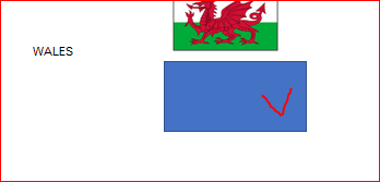
If XLOOKUP is available for you Excel, you may handle empty cells with it. First, add dummy picture at the end of your range with flags (in general it could be in any other place), like

I take blue to make it visible, after testing it could be change on any transparent shape of any form.

Next, add named formula as

=XLOOKUP('Linked Picture'!$O$28, 'Linked Picture'!$Z$31:$Z$46, 'Linked Picture'!$AA$31:$AA$46,'Linked Picture'!$AA$47)

Last parameters indicates what to return if nothing is found. I named it GetFlag. If country exists it gives

If empty cell with country name

Please check in attached file.

[#9]

Thank you Sergei. I will try - I am not very advanced with this stuff! I have looked a bit but don't see how it can work as the Getflag is different from my FlagLookups (1 for each team). I was hoping I could do something like this:
input results in R6 and S6
gives me a value in L16 then
in L17 something like
=XLOOKUP(L16,Z31:Z46,AA31:AA46,"",0,)
I know this can lookup the value of L16 and check it against Z31:Z46 but then I want it to insert the matching flag to L16 or return nothing if L16 is empty. I know I can not just stick in AA31:AA46 and the rest as I have done here in my example. Anyway, I will keep thinking about it. Very many thanks for your help. Dennis

[#10 · Accepted solution]

@DennisMetro 

You may add named formulas for each cell with flag, e.g. for L17

=XLOOKUP('Linked Picture'!$L$16, 'Linked Picture'!$Z$31:$Z$46, 'Linked Picture'!$AA$31:$AA$46,'Linked Picture'!$AA$47)

and for O17

=XLOOKUP('Linked Picture'!$O$16, 'Linked Picture'!$Z$31:$Z$46, 'Linked Picture'!$AA$31:$AA$46,'Linked Picture'!$AA$47)

[#11]

Sergei, Thank you very much indeed. That works quite well. I will have to look at it in details to try to understand but I think I know how it ties up with the linked cell. I found that the place holder is best made the same colour as the empty background. Adjusting the transparency of the placeholder, say to 0, means the inserted image when the score is known is also transparent. At any rate you've helped me reach a more satisfying outcome. Although I understand a bit in Excel I always have a feeling that there is a better way or an easier, more logical way that I don't know. For example I still have to work out the underlying facts about linking graphics and the size compared to the cells; trying to make the placeholders a bit smaller in relation to the graphic being linked; and checking to see if when a result is entered and a subsequent game is populated with new teams - the names go in but the format doesn't. I'm guessing that to have the correct format the team names would also have to be treated almost like another set of graphics.
Anyways, thank you again very much for your knowledge and help. Dennis

[#12]

@DennisMetro , you are welcome, glad it helped.

That's bit more practice, try with different variants for better understanding how it works. In general not a rocket science.