Excel Formula to find and place Unique Value, calculate days between the first entry and last entry

[bxsilva1740]

In the table below I require to find formula to fill out column C and D, since I have thousand of records to filter through

COLUMN A has duplicate ID which I need to identify the distinct ID in COLUMN D as shown
Number of days for each distinct ID from start to finish which is in Step Date (column B)
example: 10000523052 is from 4/30/2020 - 7/27/2020 = 88 days; For every Unique ID, Days(Last Entry date - First Entry Date)
I want this identified for each ID in column D as shown.

What should be the formula for Column D and Column C to show Unique ID and days between first entry and last entry for the specific ID at the top entry?

A	B	C	D
ID	Date	Distinct ID	Days
10000523052	7/27/2020	10000523052	88
10000523052	7/27/2020
10000523052	7/27/2020
10000523052	4/30/2020
10000523052	4/30/2020
10000523088	7/28/2020	10000523088	89
10000523088	7/28/2020
10000523088	7/15/2020
10000523088	4/30/2020
10000523088	4/30/2020

Thanks for your help in advance.

[#2]

@bxsilva1740 

Here's a method. I'll be curious if other more elegant solutions are proposed.

This does presume that you've sorted all of the records by the first column (the ID)... Assuming that's the case, then this formula

=IF(A3<>A2,A3,"")

will populate column C with the new ID each time it changes; otherwise leave it blank.

And then, for each row in column C that has a new ID, this formula in column D subtracts the minimum date from the maximum date for the ID in the adjacent column.

=IF(C3="","",MAXIFS($B$3:$B$11,$A$3:$A$11,C3)-MINIFS($B$3:$B$11,$A$3:$A$11,C3))

See the attached

[#3]

@bxsilva1740 

Here's a more elegant solution, in that it will list all the Unique IDs all bunched together...you could even put these formulas on their own page, apart from the database itself.

The use of UNIQUE does require the most recent edition of Excel. If you have that edition, you will find this preferable to the prior solution.

Put this wherever you want it. I illustrate it in Column C, but it could be placed elsewhere.

=UNIQUE(A3:A11)

UNIQUE will "spill" the results down as far as necessary to produce a complete list, so there should be no other content below it.

This formula remains as it was before, and should be adjacent to the foregoing.

=IF(C3="","",MAXIFS($B$3:$B$11,$A$3:$A$11,C3)-MINIFS($B$3:$B$11,$A$3:$A$11,C3))

[#4]

@mathetes  Thanks Mathetes. the suggested formula did not work; the result of the formula was 0.

Also looking for a formula for D3 to compute the number of days between the first date for the ID and last date for the same ID.

[#5]

@bxsilva1740 If you are on a modern version of excel, perhaps the attached sheet answers your question.

[#6]

@bxsilva1740 

In your file ID are numbers, and Distinc ID are texts first character of which is non-breaking space (unicode 160), most probably they are copy/pasted from Web.

For this concrete sample that could be fixed as

=MAXIFS($B$3:$B$11,$A$3:$A$11,SUBSTITUTE(C3,UNICHAR(160),"")*1)-
MINIFS($B$3:$B$11,$A$3:$A$11,SUBSTITUTE(C3,UNICHAR(160),"")*1)

[#7]

@bxsilva1740

I attached spreadsheets in both cases that DID work. I just posted the formula to make the posting more educational.

The second example, using UNIQUE, will not work, as I said, unless you have the newest versions of Excel.

[#8]

Thanks Riny_van Eekelen; did not work for me. This is what I see. Not supported.

=MAX(_xlfn._xlws.FILTER(B3:B11,(A3:A11=A15)))-MIN(_xlfn._xlws.FILTER(B3:B11,(A3:A11=A15)))

[#9]

@bxsilva1740 

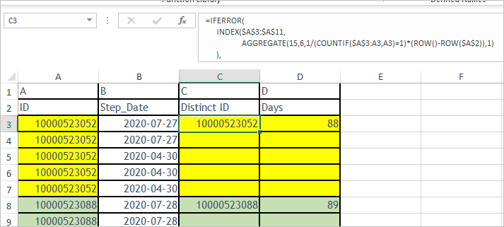
As variant

C3:
=IFERROR(
  INDEX($A$3:$A$11,
        AGGREGATE(15,6,1/(COUNTIF($A$3:A3,A3)=1)*(ROW()-ROW($A$2)),1)
  ),
"")

D3:
=IFERROR(
  AGGREGATE(14,6,1/(COUNTIFS(C3,$A$3:$A$11))*$B$3:$B$11,1)-
  AGGREGATE(15,6,1/(COUNTIFS(C3,$A$3:$A$11))*$B$3:$B$11,1),
"")

and drag down

[#10]

Thanks for your reply; works great.

[#11]

Thanks; works great.