Excel formula similiar to texjoin

[Carlo74]

hy all

I need help if is possible.

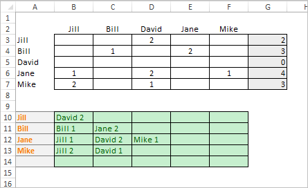
I need formula to read a complete row and when find data combine it with cell name where data is found, and to skip blanks and zeroes, and move on to next

tnx

[#2]

@Carlo74  are you use the "& "or not because this is use as  jointed before that & also good from Concatenate_Range

[#3]

@Carlo74 

I didn't catch you'd like to join result in one string or keep in separate cells as in your screenshot. If the  latest like

I'd add helper column as here in Column G (could be in any other place). In A10

=IFERROR(INDEX($A$3:$A$7,AGGREGATE(15,6,1/($G$3:$G$7>0)*(ROW($A$3:$A$7)-ROW($A$2)),ROW()-ROW($A$9))),"")

and drag it down till empty cells appear.

In B10

=IFERROR(
   INDEX($B$2:$F$2,
      AGGREGATE(15,6,1/(INDEX($B$3:$F$7,MATCH($A10,$A$3:$A$7,0),0)>0)*
         (COLUMN(INDEX($B$3:$F$7,MATCH($A10,$A$3:$A$7,0),0))-COLUMN($A$2)),
         COLUMN()-COLUMN($A$2)
      )
   ) & " " &
   INDEX(INDEX($B$3:$F$7,MATCH($A10,$A$3:$A$7,0),0),
      AGGREGATE(15,6,1/(INDEX($B$3:$F$7,MATCH($A10,$A$3:$A$7,0),0)>0)*
         (COLUMN(INDEX($B$3:$F$7,MATCH($A10,$A$3:$A$7,0),0))-COLUMN($A$2)),
         COLUMN()-COLUMN($A$2)
      )
   ),
"")

and drag it down and to the right.

[#4]

Thank you

[#5]

@Sergei Baklan thank you,

doen't work for me yet, but I'll figure it out.

could you just explain what is in formula last part, two empty rows for A2 and A9?

=IFERROR(INDEX($A$3:$A$7,AGGREGATE(15,6,1/($G$3:$G$7>0)*(ROW($A$3:$A$7)-ROW($A$2)),ROW()-ROW($A$9))),"")

[#6]

here's my original file on second sheet @Sergei Baklan 

tnx again

[#7]

@Carlo74 

Please check adjusted to your ranges formulas in attached file.

[#8]

@Sergei Baklan ,

Thank you,

this is great realy everything is working super

[#9]

@Carlo74 , you are welcome, glad to help.

Perhaps such result could be generated directly from your source table, but that's only the guess, I didn't check the logic.

[#10]

Yes,
Now with your formula, I think it could be possible by combine those formulas.
As idea it was hard for me already to get result what I want. And I was looking too complicated solutiins.
This makes averything more simple now.
Thank you

[#11]

@Carlo74 

Dynamic array solution:

=IFERROR(FILTER(FILTER($C$3:$Z$3&$C$3:$Z$27,$B$3:$B$27=$B30),LEFT(FILTER($C$3:$Z$27&$C$3:$Z$3,$B$3:$B$27=$B30))<>"0"),"")

[#12]

@Patrick2788 ,

Thanks

this solution also works great, but I can't use dynamic formulas because it cant be inserted into a table.

I need table because flow cannot rad data outside a table.

but tnx, this is great solution, I hope I will learn to write similiar formulas one day :)