Excel Filter Function - Use Same Formula Across Multiple Cells

[NareshTakashi]

Hello,

I’m looking for some guidance on using the Excel Filter function and making it so it available to use in other cells within the same column.

I have the following formula that looks for a value in A1 and produces a list from whatever is added in there. E.g. user enters ‘Am’ and the list it returns is America, Amazon….

Formula is in say B1, Map[Name] is a list of countries…

=SORT(FILTER(Map[Name],ISNUMBER(SEARCH(Item!A1, Map[Name])),"Not Found"))

It works great, however I want the formula to work for the rows after A1 (row 1), e.g. A2 (row 2), A3 (row 3), etc. I have been trying to use OFFSET and COUNTA to somehow look at the next row down to no avail. Each row must have a country in there as mandatory field, so was thinking that would work.

Any help would be really appreciated. A caveat would be that I can't use VBA! Thanks.

[#2]

@NareshTakashi  I don't understand what you mean by "work for the rows after A1".  Do you mean you want to have a filtered list for each value in column A or 1 filtered list base on a combination of values in A or something else?

So to have a list for each value in A you have the spillage problem but you could use TRANSPOSE() around your formula so instead of spilling down the column it spills to the right across columns

So to incorporate multiple options to create a combined filtered list you can:

=SORT(FILTER(Map[Name],ISNUMBER(SEARCH(Item!A1, Map[Name]))+ISNUMBER(SEARCH(Item!A2, Map[Name])),"Not Found"))

that is relatively easy to read but if you start to have a lot of items in column A that can get very large so you can also do this:

=FILTER(Map[Name],TRANSPOSE(MMULT(SEQUENCE(1,ROWS(A1:A3),1,0),--ISNUMBER(SEARCH(A1:A3,TRANSPOSE(CHOOSE(SEQUENCE(1,ROWS(A1:A3),1,0),Map[Name])))))),"none")

This is for 3 cells in A but can be expanded to larger number of rows in A.  NOTE: this will include any Name in Map that has any value in the col A range anywhere in that Name so if ANY included cell in the col A range is blank it will return all of the Names

[#3 · Accepted solution]

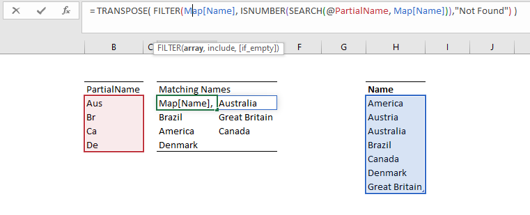
@NareshTakashi 

Conceptually, you appear to be looking to produce an array or arrays which, sadly, Excel does not traditionally support.  As was suggested, the TRANSPOSE function would allow your list of matched country names to spill horizontally, so allowing multiple lists to be stacked vertically.  This would, though, require the formula to be copied down.

Dressed up, the same formula could be written in the form

= LET(
  matches, ISNUMBER(SEARCH(@PartialName, Map[Name])),
  matchingNames, FILTER(Map[Name], matches,"Not Found"),
  TRANSPOSE(matchingNames) )

[#4]

I don't have the FILTER or SORT functions, so I can't test with those particular functions. But, you might try using textjoin to join your arrays and then filter again:

=FILTERXML("<L><I>"&TEXTJOIN("</I><I>",TRUE,IF(ISNUMBER(SEARCH(TRANSPOSE(A1:A2),MAP[Name])),MAP[Name],""))&"</I></L>","//I")

And, you'll likely need to wrap it with iferror (or some conditional test) in case none of the items exist.

[#5]

@Peter Bartholomew  @mtarler @JMB17 

Hi All,

Really appreciate your comments. Using Transpose with the formula copied down a couple of hundred rows did the job.

One thing to note, is that in my scenario I needed to Protect the sheet, to stop users messing around with the structure. In doing so, when using the filter functionality the search will chug along (my laptop is Excel 64, I7, 16GB RAM). I won't be telling users that they can filter do to this performance issue and just use the drop down.

Thanks for all your help!

[#6]

@NareshTakashi 

I wouldn't have anticipated problems especially with the machine spec you outline.

In my case, I asked for trouble by importing geographical data from the internet, so other things com into play.