Excel Date calculation formula

[MTMTMTM]

Good Morning, I'm new to this forum. I have an intermediate knowledge of Excel (Mac Office 365) and need help with a date formula. Basically, it goes like this: I have to create a payment schedule. I know the date the first payment will be made, and the date the last payment will be due. In between, I will either have 2, 3, or 4 payments. I would want the formula to take the first and last payment dates, and populate the cells in between with the due dates for the other payments. It would look something like this (total 6 payments):

                                   Due Date                  Amount

Grand Total                                                 50,000

1st Deposit.                7/20/22                   (20% of G.Total)

2nd Deposit                 Date?                     (30%)

3rd Deposit.                 Date?                     (25%)

4th Deposit.                 Date?                     (10%)

5th Deposit                  Date?                     (10%)

Final Payment.            7/20/24.               remainder?

Thanks!

MTMTMTM

[#2]

@MTMTMTM 

If you want equally spaced payments, then with 7/20/2022 in B3 and 7/20/2024 in B8, enter the following into B4 and copy into B5:B7:

=ROUND($B$3 + ROWS($B$4:B4)*($B$8-$B$3)/5, 0)

Format appropriately.  My results:

-----

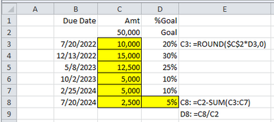
PS.... You did not ask for help with calculating payment amounts, but now I see that you wrote "remainder?".  Try the following.

[#3]

@MTMTMTM 

Try using the RandArray function in Microsoft Office 365 or 2021 to the the random dates.

Deposit	Due Date	Amount					Total Amount		Deposit	Rate
1st	7/20/2022	$10,000.00					$50,000.00		1st	20%
2nd	10/14/2022	$15,000.00							2nd	30%
3rd	8/11/2023	$12,500.00							3rd	25%
4th	10/7/2023	$5,000.00							4th	10%
5th	1/13/2024	$5,000.00							5th	10%
Final	7/20/2024	$2,500.00							Final	5%
		$50,000.00								100%

Below are the formulae. You can edit them to suit your needs.

Deposit	Due Date	Amount		Total Amount		Deposit	Rate
1st	44762	=SUM(INDEX($H$2:$H$7,MATCH(A2,$G$2:$G$7,0))*$E$2)		50000		1st	0.2
2nd	44848	=SUM(INDEX($H$2:$H$7,MATCH(A3,$G$2:$G$7,0))*$E$2)				2nd	0.3
3rd	45149	=SUM(INDEX($H$2:$H$7,MATCH(A4,$G$2:$G$7,0))*$E$2)				3rd	0.25
4th	45206	=SUM(INDEX($H$2:$H$7,MATCH(A5,$G$2:$G$7,0))*$E$2)				4th	0.1
5th	45304	=SUM(INDEX($H$2:$H$7,MATCH(A6,$G$2:$G$7,0))*$E$2)				5th	0.1
Final	45493	=SUM(INDEX($H$2:$H$7,MATCH(A7,$G$2:$G$7,0))*$E$2)				Final	=$H$8-SUM(H2:H6)
		=SUM(C2:C7)					1

Note:

Because the i used the RandArray function the dates keeps changing so you can copy the dates and paste as values in the same cells or you can even use macro to do that.

Also, remember to format the Due dates column as date.

Other contributions or inputs are welcome

Hope you find this helpful

Thanks

@DonShearer

[#4]

Please below is the formula for the Due Dates using RandArray function.

For the Due Dates column as date

Deposit	Due Date	Amount		Total Amount		Deposit	Rate
1st	44762	=SUM(INDEX($H$2:$H$7,MATCH(A2,$G$2:$G$7,0))*$E$2)		50000		1st	0.2
2nd	=SORT(RANDARRAY(COUNTA(A3:A6),1,B2,B7,TRUE))	=SUM(INDEX($H$2:$H$7,MATCH(A3,$G$2:$G$7,0))*$E$2)				2nd	0.3
3rd		=SUM(INDEX($H$2:$H$7,MATCH(A4,$G$2:$G$7,0))*$E$2)				3rd	0.25
4th		=SUM(INDEX($H$2:$H$7,MATCH(A5,$G$2:$G$7,0))*$E$2)				4th	0.1
5th		=SUM(INDEX($H$2:$H$7,MATCH(A6,$G$2:$G$7,0))*$E$2)				5th	0.1
Final	45493	=SUM(INDEX($H$2:$H$7,MATCH(A7,$G$2:$G$7,0))*$E$2)				Final	=$H$8-SUM(H2:H6)
		=SUM(C2:C7)					1

Deposit	Due Date	Amount		Total Amount		Deposit	Rate
1st	7/20/2022	$10,000.00		$50,000.00		1st	20%
2nd	9/8/2022	$15,000.00				2nd	30%
3rd	4/20/2023	$12,500.00				3rd	25%
4th	8/7/2023	$5,000.00				4th	10%
5th	5/12/2024	$5,000.00				5th	10%
Final	7/20/2024	$2,500.00				Final	5%
		$50,000.00					100%

@DonShearer 

[#5]

This is great, so helpful, thank you so much!! Very generous response, most grateful!

[#6]

THIS is awesome, thank you so much for the more than thorough response. First time in this forum, this is great!