- Subscribe to RSS Feed
- Mark Discussion as New
- Mark Discussion as Read
- Pin this Discussion for Current User
- Bookmark
- Subscribe
- Printer Friendly Page
- Mark as New
- Bookmark
- Subscribe
- Mute
- Subscribe to RSS Feed
- Permalink
- Report Inappropriate Content
Dec 10 2020 09:47 AM
How do I get Excel to turn the font red when there is a negative result to the formula?
Appreciate any assistance.
- Labels:
-
Formulas and Functions
- Mark as New
- Bookmark
- Subscribe
- Mute
- Subscribe to RSS Feed
- Permalink
- Report Inappropriate Content
Dec 10 2020 09:55 AM
Select the cell(s) with the formula.
On the Home tab of the ribbon, click Conditional Formatting > New Rule...
Select 'Format only cells that contain'.
Leave the first drop-down set to the default 'Cell Value'.
Select 'less than' from the second drop-down.
Enter 0 in the box next to it.
Click Format...
Select red as font color.
Click OK, then click OK again.
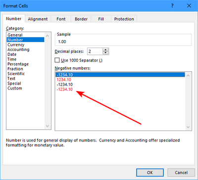
Alternatively, you can specify that negative numbers should be red in the number format of the cells. No conditional formatting rule needed.
