Excel Conditional Formatting to highlight Matches/Non matches with different colors

[DingoDigits]

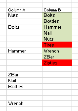
Hello, I have two columns

- Column A has unsorted items that may include one or more blank lines in between each item 

- Column B is a sorted list of items that 'should' be present in the first column.

My goal is to highlight the items in column B : green for items that exist in the column A, and red for items that do not exist in the column A.  A complexity is that the number of rows in the column B can vary greatly so I need a formula that will adjust to the number of non-blank rows in column B so I don't end up with 50 empty red highlighted cells.

I can achieve the first, green highlighting using this conditional formatting formula as the first rule: =MATCH(B2,A$2:A$200,0) (NOTE: the A$200 allows for the varying number of rows in column B), but can't seem to get a second rule that will achieve the red highlighting - without making more rows red than should be.

I'm sure it probably easy but I'm stuck so any help would be appreciated!

Thanks

[#2 · Accepted solution]

@DingoDigits 

You may use

Red:
=NOT(SUM(COUNTIF(B2,A$2:A$200)))

Green:
=SUM(COUNTIF(B2,A$2:A$200))