Excel bubble chart: how to size bubbles based on no. of items with identical x and y values?

[Tormod Solem Slupphaug]

I have a set of data with x and y columns containing values from 1 to 5. I've placed all the rows/items in a bubble/scatter chart.

The challenge:

How can I size the bubbles relative to eachother by number of items registered "per coordinate" / items with identical (x and y) values?

Example data table:

	Probability	Impact
#1	4	1
#2	4	1
#3	4	1
#4	4	2

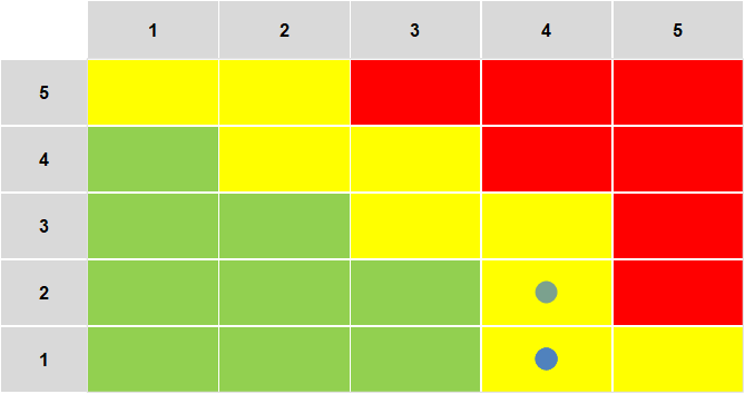
Example bubble chart (just a transparent bubble chart placed on top of coloured cells):

Since 3 items corresponds to the (4, 1) coordinate, while only 1 item corresponds to (4, 2), I want the bubble in (4, 1) to be bigger. As I add more items with other coordinates, I want the bubble chart to update automatically with relative sizes.

[#2 · Accepted solution]

@Tormod Solem Slupphaug 

A bubble needs 3 argument. You have to add a counter column:

Probability	Impact	n
4	1	3
4	1	3
4	1	3
4	2	1

Select row 2-5 (not the headers) and insert a bubble and i should be Ok (if you use a 2-D chart. In a 3D chart you will se that you have stacked 3 bubbles on top of each other).

You can create the 3:d column with 

=COUNTIFS($A$2:$A$5,A2,$B$2:$B$5,B2)

Anther way is to use a Pivot table to create something like:

Probability	Impact	n
4	1	3
4	2	1

But you cant use it in a pivotChart so it's kind of pointless

[#3]

Thanks, your COUNTIFS formula is just what I was looking for.