Example - Mechanical Inspection using AQL

[AnthonyCappuccio]

Hey Everyone,

I am looking to create conditional formatting on a range of cells that will populate said cells based off of an AQL table. I have attached the excel file that shows the data and what I am trying to do. There is a text box on "TAB 2" that explains the goal of what I am trying to achieve.

I believe I will need to use an equation to format the cells but based off prior research into excel functions - I think this formula will need to be a little sophisticated. I believe currently that the formula will need to be some variation of a nested VLookup function or possibly a VLookup nested with an HLookup.

NOTE:

The "TABLE" tab lists 'Lot Size' as ranges. Currently I am skeptical about leaving this as a range because I think it will make the equation needed even more complicated (unless this task can be performed using the approximate return of V/HLookup which I am unsure of but thought it has potential). If necessary I am open to creating a table that has one cell per one lot size (i.e. C5=2, C6=3, C7=4, etc.) in order to make this work.

[#2]

@AnthonyCappuccio 

I'd do that with helper ranges/cells. For the main table

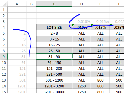
add percents as numbers, not as texts on the top, and on the left low boundary of ranges.

Here

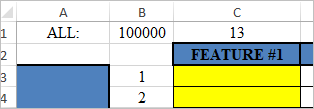
in B1 how we interpret ALL, and in C1 formula

=IFERROR(
   --INDEX(TABLE!$D$5:$S$19,
      LOOKUP('TAB 1'!$E$3,TABLE!$A$5:$A$19,(ROW(TABLE!$A$5:$A$19)-ROW(TABLE!$C$4))),
      MATCH('TAB 1'!$E$5,TABLE!$D$3:$S$3,1)),
'TAB 2'!$B$1)

and conditional formatting rule formula as

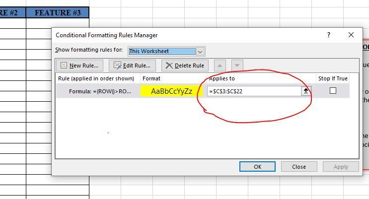
=(ROW()>ROW($C$2))*(ROW()<=($C$1+ROW($C$2)))

It could be combined al together in one formula, but it will be hard to maintain such.

[#3]

@AnthonyCappuccio don't forget to update the cells the formatting will apply to in case you have a situation when the value is greater than 20.

 @Sergei Baklan is there a reason why the iferror function should return "Tab2 B1" which has 100,000 as its value? 

[#4]

@Sergei Baklan 

Sergei - Thank you for taking the time to explain this so thoroughly. I am not nearly this experienced in Excel so to come up with this would be near impossible for me. I really do appreciate the help!

A few questions:

1. When you say it would be hard to maintain this as one formula are you referring to excel's ability to maintain it and process the formula within the formatting?
2. Also, I did not mention this on the post but another key aspect of this whole thing is that I need the yellow cells to turn back to white after information is manually inputted. Meaning after the Quantity and AQL are entered on TAB 1, the purpose of this sheet will be for a mechanical inspector to input data into these yellow cells based on a tolerance range for a feature. Upon entering the value into the yellow cell on TAB 2 I would need the cell to then change from yellow to white signifying data has been entered.
3. Is this an easy addition given the way you had written the formula on the excel file you had provided?

@wumolad  Thanks for the heads up. I had taken this into consideration - I didn't want to complicate this example file too much but I definitely will be extending this past 20 pieces!

[#5]

@wumolad 

No reason except that shall be some number to apply formatting. I know nothing about that business and have no idea that ALL could mean on practice.

[#6]

@AnthonyCappuccio 

1) It'll be much harder to change the formula and much longer to develop it. If you don't like to have all these additional cells together with main data, such data preparation calculations could be moved on separate sheet (both table helper columns and intermediate calculations) and such sheet could be hided not to show it to end user.

2) Not to color cells with data we may check if the cell is empty or not by one more criteria

=(ROW()>ROW($C$2))*(ROW()<=($C$1+ROW($C$2)))*(C3="")

3) Not sure I understood this question, could you please clarify a bit.

[#7]

@Sergei Baklan 

Thank you for the suggestion. I will most likely end up adding the formula to the sheet where the table is located as the sheet involving the recording of the feature will have to maintain a certain appearance that will need this hidden.

The new formula you updated for #2 was exactly what I was looking for. I was trying to ask you (in question 3) if adding the step about switching from yellow to white when data is entered would be difficult based on what you initially provided but I see now how you included it.

.

.

One question I have regarding ALL:

As I'm messing around with the file you sent I'm noticing when a value for AQL and Quantity are chosen that correlate to "ALL" in the TABLE - this results in all 20 piece #'s flagging yellow. How would I alter this so that "ALL" in the TABLE tab is reflective of the Quantity entered on TAB 1?

[for example] The attached filed I added, the Quantity is 5 and AQL is 0.01%. From the table this is defined as ALL and TAB 2 highlights all 20 piece #'s listed on TAB 2. In this case there are only 5 parts in the quantity so ideally only 5 piece #'s would need to be highlighted on TAB 2.

Essentially the connection I am making is if ALL is the chosen cell from the TABLE then the highlighted cells would be reflective of the exact quantity indicated on TAB 1.

This is where I mentioned in the original post that I was skeptical about ranges and considered making this table much larger to include one number per lot size in fear of this exact need being to complex.