Embedded CONCAT in AVERAGE function results in #VALUE! error

[Lucky7423]

I'm trying to dynamically put a variable range of cells in an AVERAGE function to cover different periods preceding the most recent.  In this approach I would only have to change the last row number (in this case 2820 in C2839) instead of recalculating and changing each AVERAGE formula.  I have tried numerous approaches but can't seem to rid the result of quote characters which show up during an Evaluate Formula but don't show in the CONCAT cell itself.  It may be something simple I'm overlooking but at this point I could use some help.  GRProbA shows the normal view; GRProbB shows the formulas.

[#2]

Hello @Lucky7423  ,

You cannot just create a text string and use that like a range reference. You need to convert the text to a range with the Indirect function. So, if cell E2 contains a formula that returns "A1:A4" as a text, then you can use

=AVERAGE(INDIRECT(E2))

Or you can build the concatenation right into the Indirect function

=AVERAGE(INDIRECT(C2&C3&":"&C4&C5))

Screenshot to illustrate:

[#3]

another approach is to use Offset() instead of Indirect() to create a variable range. The syntax for Offset is

Offset(StartRange,rows,columns,height,width)

Offset(A1,0,0,4) will generate a range that starts at A1, goes 0 rows down, 0 columns to the right (i.e. it anchors at A1), is 4 rows high and, since no width is specified, has the same width as the first parameter (A1, so 1 column wide). 

=AVERAGE(OFFSET(A1,0,0,4))

Change the first parameter to modify the start date and change the height parameter to return more rows. 

[#4]

@Lucky7423 

Just to add to @Ingeborg Hawighorst's posts, it should be pointed out that volatile INDIRECT and OFFSET set-ups can almost always be replaced with a non-volatile INDEX one in such cases.

For example, the following are all equivalent:

=AVERAGE(C1:INDEX(C:C,A1))

=AVERAGE(INDIRECT("C1:C"&A1))

=AVERAGE(OFFSET(C1,0,0,A1))

though only the first is non-volatile (well, not quite: technically volatile just once, i.e. when the workbook is first opened, but for all intents and purposes that's non-volatile).

Regards

[#5]

@Ingeborg Hawighorst  THANK YOU! Problem solved!

[#6]

@Jos_Woolley  Thank you for responding. Seeing your three examples together is helpful.

[#7]

@Lucky7423 

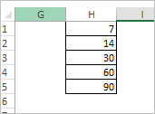
One more point - it looks like you calculate the same range sizes. They could be defined in any helper range, e.g.

And if in A1 the last row to use, e.g. 2820, formula for 7 days average could be, as suggested earlier,

=AVERAGE(INDEX(D:D,$A$1-$H1+1):INDEX(D:D,$A$1))

and drag it down to receive another 4 averages.