Dynamic MATCH 2D array with one-cell spilled formula

[leolapa]

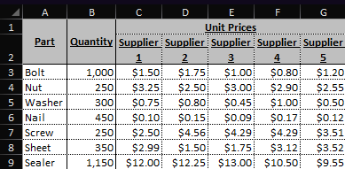
I've got the sample table below with a list of parts/quantities and respective price quotes from 5 dummy suppliers:

What I need to accomplish here is to automatically generate a separate table that will rank all suppliers by price (from lowest to highest) for each part row.

But since this is a dynamic sheet that may grow either in number of quoted items and/or suppliers, I need this formula 2D dynamic that "spills" the results down the list of items and across the ranked suppliers for each item.

This is something I was able to accomplish using a 3-step approach detailed on the screenshot below:

Each step is detailed on the blue, orange and yellow sections above.

The yellow part is the result I want to get, and in both blue and yellow I managed to do so by inputting a formula in one cell only (I3 and U3 respectively) and Excel spill the results down and across for me - I won't bother with the details of both formulas...

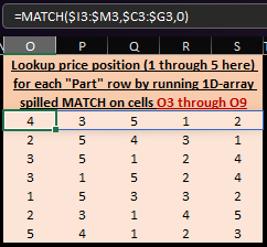
The middle orange part, the 2nd step is the one I'm having trouble with since MATCH in itself works only with one-dimensional arrays, as per the screenshot below:

In order for this formula to work I'd always need to copy/paste down every time new items are added to the quote table, as it only covers growth on number of suppliers across.

I've tried a couple different approaches using RANK and BYROW but to no avail, any help is appreciated here...

I also attached the Excel file that produces the above screenshots.

Thanks in advance!

[#2 · Accepted solution]

@leolapa I formatted your data as a Table and then used this:

=LET(h,DROP(PartTable[#Headers],,2),
     s,SEQUENCE(1,COLUMNS(PartTable)-2,3),
     REDUCE(s-2,SEQUENCE(ROWS(PartTable)),
        LAMBDA(p,r, VSTACK(p,SORTBY(h,INDEX(PartTable,r,s))))))

see attached

[#3]

Very clever solution @mtarler!

I knew a LET/LAMBDA type approach would do the trick, but I couldn't quite get there as I still need to brush up my skills on that arena.

Thanks