Dynamic Drop Down Lists

[Jon_R1968]

Hi,

I'm trying to set up a multi row schedule whereby once a selection is made from a Drop down list in Column B it automatically identifies the relative options in a Drop Down list in Column C (all info for the  Drop Down lists sourced from a table in a separate worksheet.

I've had a go at it in the attached example workbook but feel it is a little Heath Robinson and probably unstable? (it generates numerous Circular reference errors) - I've tried to use the address of the active cell to generate the information in Column C's Drop Down list but not sure if this is the best or correct way to resolve this challenge. Ideally there is an Excel Formula solution as I have no experience of VBA or Pivot tables.

Any advice would be much appreciated.

Cheers

[#2 · Accepted solution]

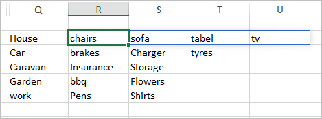
@Jon_R1968 

You may prepare data for it as

with

=TRANSPOSE(FILTER(Table1[Item],Table1[Location]=$Q2))

and use for data validation in column C

=XLOOKUP($B2,Data!$Q$2#,Data!$R$2:$R$6)#

[#3]

@Sergei Baklan 

Thank you for your advice and updating my workbook. I'll review all at work tomorrow and advise if any further queries or if your kind response has resolved everything.

Thanks again

@Jon_R1968 

[#4]

@Jon_R1968 

Excel always (well, almost always) gives us multiple ways to accomplish the same fundamental task.

Here's an example of yet another way to have a secondary data validation (or drop-down) which changes based on the selection of the first.

[#5]

@Sergei Baklan 

Thank you. Your solution has worked a dream. Being honest, I'm not quite sure how the various functions in the formulas you provided work but they do!......it gives me something to work on in developing my knowledge.

Thanks again

[#6]

@mathetes 

Thank you for taking the time to respond to my query. I had previously started working on the solution @Sergei Baklan provided (which worked) and thus haven't used your solution but do appreciate your input.

Thanks again

[#7]

@Jon_R1968 , you are welcome.

I'm not sure where this pattern is explained in details, but if you have concrete questions please ask.