Dynamic Average based off the position of the first non-zero data point

[krisplikj]

Hello,

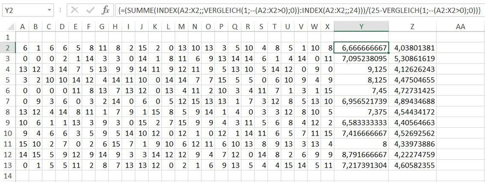
This is piggy-backing off a previous question that was solved in finding the number of "leading zeroes" in monthly sales data.  I am looking at the previous 24 months (columns a:x) and then column y counts the number of leading zeroes when present.  For example,

Row 2 = (100,50,150,0,125,100,etc) the number of leading zeroes in column Y is zero

Row 3 = (0,0,50,0,100,200,300,etc) the number of leading zeroes in column Y is two

What I want to do is calculate the average, standard deviation, etc with varying starting points by row, based off where the first "non-zero" occurred.  In row 2, the first non-zero occurred in column a.  In row 3, the first non-zero occurred in column c.  Thanks all!

[#2]

@krisplikj 

=(SUM(INDEX(A2:X2,,MATCH(1,--(A2:X2>0),0)):INDEX(A2:X2,,24)))/(25-MATCH(1,--(A2:X2>0),0))

For the average calculation you can try this formula. Enter the formula with ctrl+shift+enter if you don't work with Office365 or Excel 2021. 

=STDEV.P(INDEX(A2:X2,,MATCH(1,--(A2:X2>0),0)):INDEX(A2:X2,,24))

This is the formula for the standard deviation in cell Z2. Enter the formula with ctrl+shift+enter if you don't work with Office365 or Excel 2021. 

[#3 · Accepted solution]

Hi @krisplikj 

With 2021 or 365:

AVERAGE in Y2:

=AVERAGE(XLOOKUP(TRUE,A2:X2<>0,A2:X2,X2):X2)

[#4]

Thanks LZ! This is perfect. Much appreciated!

[#5]

Thanks Pawn! This worked. An alternate solution provided which also worked was =AVERAGE(XLOOKUP(TRUE,A2:X2<>0,A2:X2,X2):X2)

Happy holidays to you and yours.

[#6]

Glad this helped & Thanks for providing feedback

[#7]

@krisplikj 

You are welcome. Instead of the long-winded formula i originally suggested for average one can apply this formula:

=AVERAGE(INDEX(A2:X2,,MATCH(1,--(A2:X2>0),0)):X2)

However since you have access to XLOOKUP the solution by @L z. is the best way for this.

Happy holidays to you and yours as well.