- Subscribe to RSS Feed
- Mark Discussion as New
- Mark Discussion as Read
- Pin this Discussion for Current User
- Bookmark
- Subscribe
- Printer Friendly Page
- Mark as New
- Bookmark
- Subscribe
- Mute
- Subscribe to RSS Feed
- Permalink
- Report Inappropriate Content
Sep 30 2022 09:18 PM
Hi,
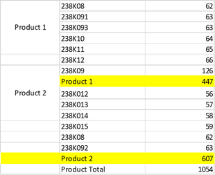
I have create a dynamic array and then add a value column in the left that array. The column contains 2 values "Product 1" and "Product 2" that is merged cells, they are hard data. The issue is when dataset is added, the array is updated but the hard data is not moved respectively.
Maybe, have some ways to approach that.
I have added an image and the samplefile below.
Can you give me some advices.
Thank you.
- Labels:
-
Excel
-
Formulas and Functions
- Mark as New
- Bookmark
- Subscribe
- Mute
- Subscribe to RSS Feed
- Permalink
- Report Inappropriate Content
Sep 30 2022 10:33 PM
Solution@littlevillage I feel like you were on the right track. Merged cells are quite static and, as such, shouldn't be paired with dynamic arrays where the range will constantly change.
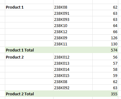
Since your dynamic array is based off the pivot table, I used a label filter to remove any id's containing product. Instead, I used the subtotal (as I noticed when I added additional rows to the source of the pivot table, obviously the values of product 1 & product 2, etc, would not update to reflect the new rows).
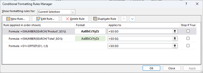
For the formatting, I used your approach with slightly different formulas:
Workbook is attached for your reference.
Hope this helps.
Dexter
- Mark as New
- Bookmark
- Subscribe
- Mute
- Subscribe to RSS Feed
- Permalink
- Report Inappropriate Content
Oct 01 2022 07:54 AM
Thank you very much.
The OFFSET function is as key for the formula.
It actually worked.
Regards,
Phan.
Accepted Solutions
- Mark as New
- Bookmark
- Subscribe
- Mute
- Subscribe to RSS Feed
- Permalink
- Report Inappropriate Content
Sep 30 2022 10:33 PM
Solution@littlevillage I feel like you were on the right track. Merged cells are quite static and, as such, shouldn't be paired with dynamic arrays where the range will constantly change.
Since your dynamic array is based off the pivot table, I used a label filter to remove any id's containing product. Instead, I used the subtotal (as I noticed when I added additional rows to the source of the pivot table, obviously the values of product 1 & product 2, etc, would not update to reflect the new rows).
For the formatting, I used your approach with slightly different formulas:
Workbook is attached for your reference.
Hope this helps.
Dexter


