Duplicate Columns

[RileyTim184]

So, I'm new to using Excel and I've been trying to figure something out. I'm doing an Excel sheet of people who donated to a fund with their names and the amount they donated.

My issue is there are about 5,000 rows of people and most of these are duplicates names. (For example, if their name is John Smith their name will come up multiple times if they donated multiple times) Their names are column "A" and the amount they donated is column B.

The donation totals are supposed to be aggregated (that if someone made separate donations I add them together and just have one line per individual- with their total) Is therean easier way to do this without having to manually add all the donations?

I'm trying to add up John Smith's for example donation totals without having to do it all by hand. I didn't know if Excel was able to add these totals together for individual people. The screenshot isn't the actual Excel sheet I'm doing, just an example I made up. Thanks for any help.

[#2]

@RileyTim184 The easiest way out would be to use a Pivot Table. See the attached workbook for a working example.

Search the web for many resources to learn more about Pivot Tables.

[#3]

@RileyTim184 

If you are using Excel 365, there are some newish worksheet functions that will also do the job.  Given the two columns 'name' and 'donation', a list of distinct names is given by the formula

= UNIQUE(name)

and then the donations for each distinct name are given by

= SUMIFS(donations, name, distinct#)

[Note: If the name 'distinct' is applied to the first cell containing the formula, 'distinct#' will be its spilt range)

[#4]

@Riny_van_Eekelen Oh great thank you! I didn't know I could do this. Very helpful.

[#5]

Thank you for your help! I will try this out.

[#6]

@Riny_van_Eekelen 

I'm trying to figure out the Pivot table and I'm having a little trouble.

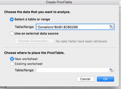
The 'Donations!$A$1:D ....." screenshot is what pops up first when I hit the pivot table.

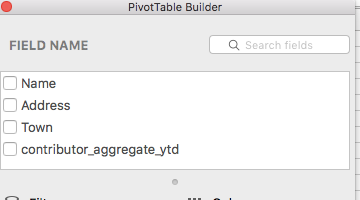
There's an A, B, C, and D column for their name, address, town, and how much they donated. A is the name column and B is the donations like I said earlier. 

I hit the "Ok" button and I checked the name and aggregated ytd (aka donations) boxes.

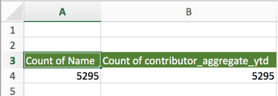
The issue I'm having is I think it's adding the columns altogether (added the screenshot to show)

Am I missing a step? Do I have to highlight a certain section before hitting the pivot table button or do I have to put in something different under the "Select a table or range" part at the "Create PivotTable box? Thanks.

[#7]

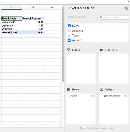
@RileyTim184 From your screenshots I can see you're on a Mac. So, am I. That makes it easier to explain. When you created the table, you dragged both Name and Donation into the "Value field". Drag the Name into the "Rows" field (red arrow). 

Now press the (i) to the right of where it says "Count of Amount" (blue arrow). It should look like this;

You'll ses the "Count" is highlighted in the "Summarise by" box. Select "Sum" to tell Excel you want to add up the amounts, not count them. The end result will look like this (use the file I uploaded with my initial response as a reference):

Now, if you never got this far and Excel defaulted to count amounts, it means that your list of donations contains texts. They may look like numbers, but they are not. Then you need to fix that first. To see if your amounts are (or contain) texts, put the formula =ISNUMBER(D2) in E2 and copy it all the way down. If anywhere it returns FALSE you'll find your text. Let me know your findings.

[#8]

It worked! Thank you so much, I really appreciate it. You just saved me so much time, thanks again.