Does anyone know how to: Cell A1 = Cell A2, enter (checkmark) in Cell A3?

[dcb12204]

And if not equal, enter an "X"?  I tried inserting symbols and wingdings in an IF statement, and could not get them to work.  Only normal text would work.  Please help.

[#2]

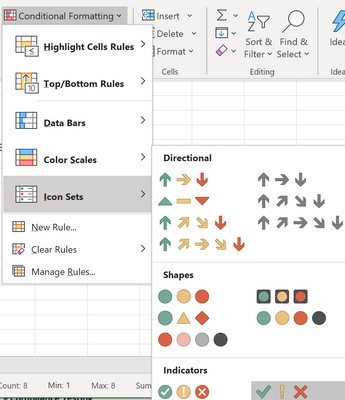
@dcb12204  this seems like a good use for conditional formatting:

You can create that extra column with some default values (0,1) and then apply the conditional formatting to that column.  BTW you can make the font white or background color so the text isn't visible and/or make the column very narrow so that check mark/ X hides the text. 

[#3]

@dcb12204 

If I am allowed, I would like to add two quick and simple solutions to the elegant solution from Mr, Mr,mtarler  .
1. = IF (A1 = A2, "", "X")
2. = IF (A1 <> A2; ”X”; ””)

3. Insert tick without conditional formatting and VBA:
if you use check boxes from the "Controls Toolbox" toolbar, you can connect them to a cell in the worksheet. After inserting the check box, you are initially in design mode. In this mode you can set the properties of the check box by right-clicking on the box and selecting the "Properties" item in the pop-up menu. If you look at the property "LinkedCell" e.g. Write A1 in, cell A1 is linked to the box, i.e. if the check box is selected, the cell reads "True", otherwise "False". Now you can query the cell in the formulas instead of the check box.

Hope I was able to help you.

Nikolino

I know I don't know anything (Socrates)

[#4 · Accepted solution]

@dcb12204 

As variant that could be like

[#5]

@Sergei Baklan

Wow.  That is quite the formula.  I have never seen one constructed quite that way.  Can you explain how the structure works for me? 

[#6]

@dcb12204 

For your purposes you may use two inicode characters with codes 10004 and 10006. That's only one condition, one cell is equal to another or not, based on which you take one or another code.

Logical TRUE and FALSE in calculations are equivalent to 1 and 0 accordingly. Thus

10004+2*(A1<>B1) is equal to 10004+2*(FALSE) = 10004+2*0 = 10004

or

10004+2*(A1<>B1) is equal to 10004+2*(TRUE) = 10004+2*1 = 10006

[#7]

@dcb12204 

There is another technique that works.  Building on @Sergei Baklan 's solution. one could simply use the formula

=N(A1=B1)

[which gives 0 or 1] in combination with the number format

✔;✔;✖

or even

[Blue]✔;✔;[Red]✖

if you want to get fancy!