Data validation range based on another cell contents

[Brirack77]

Hi All,

I am having trouble with this one and feel like it should be easier than it is (for me)

I want to have two data validation columns, Column C is whole no. 1 thru 6, Column D is a range % BASED on the result in Column C. So if C2 = 1, D2 only offers an input of 0%. However if C3 = 4, D3 offers an input of between 100% & 130%. This could be as a dropdown on just valid range between min & max.

Example attached and thank you.

[#2 · Accepted solution]

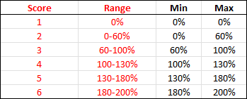
@Brirack77 

Split the min and max values into separate columns:

Next, select D5:D10.

On the Data tab of the ribbon, click Data Validation.

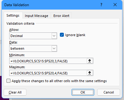
Select Decimal from the Allow drop down, and between from the Data drop down.

In the Minimum box, enter the formula =VLOOKUP(C5,$C$15:$F$20,3,FALSE)

In the Maximum box, enter the formula =VLOOKUP(C5,$C$15:$F$20,3,FALSE)

If desired, activate the Input Message and Error Alert tabs and enter appropriate messages.

Finally, click OK.

See the attached workbook.

[#3]

works a treat thank you! (I did a lot of named ranges to not get this to work in another way :\ )

[#4]

@Hans Vogelaar 

Question.. I have a similar issue.  in one cell the user is going to select a "location" and based on that location, I need the validation to move from one set of options to the next... I.E. if C2 = "OH", then use the list between D1:D20, if C2="TN" then use the list between E1:E50, if C2="NC", then use the list between F1:F15, if C2="KY" then use the list between G1:G6.   Each location has a specific areas that can be chosen from and based on what area they are in, want to limit the validation to their specific choices.  Is this possible?

[#5]

@AOSPWB 

That is called a dependent data validation drop-down. It requires a different technique.

See Create Dependent Drop-Down Lists 

[#6]

Thank you! Works rather well. Only one item I am trying to understand... I needed to make the list include a few 'blanks' so that we can add on the second drop down and now, after selecting the "site", when going to the next one, sometime when I click on the pull down, it will start by showing the first in the list and sometimes it starts with the blanks which requires me to scroll to the top. The "Ignore" blanks is selected. also - any reason the auto complete is not working? I.E. on the Using Ohio instead of OH as the actual name.

[#7]

@AOSPWB 

If you include blanks in the list (which I don't recommend), and if the active cell is blank, Excel will select the first blank in the list when you click the drop-down arrow. If the cell is not blank, Excel will select the current value in the list.

Which version of Excel do you use?

[#8]

apologies for delay - 'life'.... we are using office 365 and I have blanks in the table because I am trying to allow this thing to grow as we need it and I know each site will have areas added and easier for someone to pick a blank, type in a new option than try to redo lists, etc. But if it is going to cause massive issues, then I will eliminate the blanks and my team will just need to monitor.

[#9]

So, I have taken out the blanks in the tables so that is no longer an issue, but any reason why the "autocomplete" is not working? Be great if they could start to type and it would give suggestions to help speed up the process.

[#10]

@AOSPWB 

Select File > Account.

What do you see next to "About Excel"? On my PC, it is

[#11]

Version 2302 (Build 16130.20846 Click-to-Run)
Semi-Annual Enterprise Channel

[#12]

@AOSPWB 

That explains it. AutoComplete was introduced in version 2308.

Your version is older. You'll have to wait until you are updated to 2308.

[#13]

its not just me then... if this file is to be used by others, I really need to wait until ALL are updated to that vs. Appreciate the insight! Not what I was expecting nor what I like, but it is what it is and guess I am at the mercy of whatever dept controls the updates, etc. Sure it is a lovely dept wrapped in red tape