- Home
- Microsoft 365
- Excel
- Re: Creating a training matrix from a dataset
Creating a training matrix from a dataset
- Subscribe to RSS Feed
- Mark Discussion as New
- Mark Discussion as Read
- Pin this Discussion for Current User
- Bookmark
- Subscribe
- Printer Friendly Page
- Mark as New
- Bookmark
- Subscribe
- Mute
- Subscribe to RSS Feed
- Permalink
- Report Inappropriate Content
Mar 13 2021 09:19 AM
Trying to create an employee training matrix from a dataset of employee training records. A simple pivot table would suffice if only it would insert the "course date" as text, and not summarize it as either count/sum. Are tables the solution? Some other tool? I manually transferred the below data (left) to the desired matrix format (right), below.
- Labels:
-
Charting
-
Excel
-
Formulas and Functions
- Mark as New
- Bookmark
- Subscribe
- Mute
- Subscribe to RSS Feed
- Permalink
- Report Inappropriate Content
Mar 13 2021 09:21 AM
Dataset:
| Name | Course | Course Date |
| Smith | WHMIS | 15/03/2020 |
| D'Amico | Working at Heights | 20/02/2016 |
| D'Amico | Asbestos | 25/04/2019 |
| Culbertson | Basics of Supervising | 04/02/2020 |
| Culbertson | Lockout & Tagout | 17/07/2016 |
| Culbertson | WHMIS | 31/03/2019 |
| Culbertson | Asbestos | 19/03/2020 |
| Culbertson | Working at Heights | 04/05/2019 |
| Mastroluisi |
- Mark as New
- Bookmark
- Subscribe
- Mute
- Subscribe to RSS Feed
- Permalink
- Report Inappropriate Content
Mar 13 2021 10:24 AM - edited Mar 13 2021 12:15 PM
Solution
Two methods.
First:
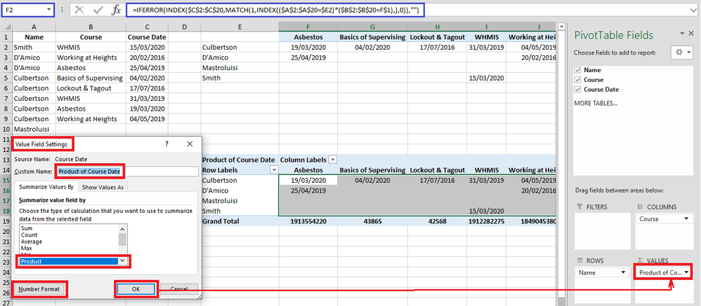
With Pivot Table. Click one of the cells of your data (for example cell A2) and then create a Pivot Table in same sheet when you are working. In my example I have created it in cell E13.
- Draw the fields as I have made (see the printscreen).
- In the VALUES box right click on Count of Course Date and in Value Field Settings choose Product.
- Select cells F13:J18 and format them as date.
Second:
In colum E create a list with unique names.
In cell F2 apply below formula:
=IFERROR(INDEX($C$2:$C$20,MATCH(1,INDEX(($A$2:$A$20=$E2)*($B$2:$B$20=F$1),),0)),"")
drag it right and than down. Format cells F2:J5 as date.
You can download my file at this link: https://1drv.ms/x/s!Ah_p7p0xkR5RnWoDDtSELLY1zuHA?e=pfd5SJ
Hope this hepls.
Regards,
IlirU
- Mark as New
- Bookmark
- Subscribe
- Mute
- Subscribe to RSS Feed
- Permalink
- Report Inappropriate Content
Mar 13 2021 01:31 PM
Accepted Solutions
- Mark as New
- Bookmark
- Subscribe
- Mute
- Subscribe to RSS Feed
- Permalink
- Report Inappropriate Content
Mar 13 2021 10:24 AM - edited Mar 13 2021 12:15 PM
Solution
Two methods.
First:
With Pivot Table. Click one of the cells of your data (for example cell A2) and then create a Pivot Table in same sheet when you are working. In my example I have created it in cell E13.
- Draw the fields as I have made (see the printscreen).
- In the VALUES box right click on Count of Course Date and in Value Field Settings choose Product.
- Select cells F13:J18 and format them as date.
Second:
In colum E create a list with unique names.
In cell F2 apply below formula:
=IFERROR(INDEX($C$2:$C$20,MATCH(1,INDEX(($A$2:$A$20=$E2)*($B$2:$B$20=F$1),),0)),"")
drag it right and than down. Format cells F2:J5 as date.
You can download my file at this link: https://1drv.ms/x/s!Ah_p7p0xkR5RnWoDDtSELLY1zuHA?e=pfd5SJ
Hope this hepls.
Regards,
IlirU

