Create a chart based on a subset of the data in a table

[Michael63]

Hi,

My workbook contains two worksheets, one with the data and another one with charts. Let's say I have a scatter chart that needs to display the data based on specific filter criteria, e.g. a particular month or quarter. 

I know that I can apply a filter on the data table and the chart would automatically ignore the hidden values.

However, I don't want to touch the worksheet with the data table directly. Is there any way how to achieve this? I have experimented also with Advanced Filter but could not get this right. 

[#2]

Hello,

You can create PivotTables from the source data. Thereafter, you will create PivotChart

[#3]

A Pivot Table does not work in my case because for the Scatter chart I need all data points within a certain period. Pivot tables always aggregate.

[#4]

@Michael63 

In general you may filter the chart independently from data source, but not the scatter one. If to separate data for the chart from the source table, Advanced filter shall work, but I'd prefer to do that through data model. In any case Refresh All will be required in case of changes.

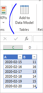
We may add data to data model from Power Pivot menu

or if it's not activated by creating dummy PivotTable with adding data to data model.

Next, form Data->Existing Connections let select the table

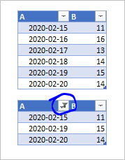
and put it in desired place in the workbook. Now we may build the chart based on this table applying to it filter independently on data source

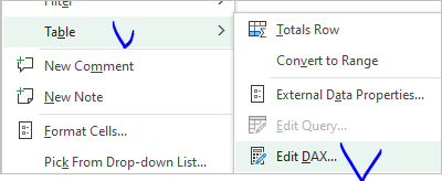
The question is how to apply filters. That could be direct filtering of the second table, slicers or some parameters defined in another range/table of the sheet. With the latest we may add them also into the data model and returned the second table not as the copy of the source, but as result of DAX expression evaluation which builds resulting table taking parameters into account.