Conversion of data into single column

[saleemch]

Hi all, I need to convert multiple columns data into one columns. The columns represent yearly flows and may have 365 or 366 values. Could any body suggest me code to convert data into one column say 1-1-1960 to 31-12-2011. Spreadsheet is attached for your reference.

Regards

Saleem

[#2]

@saleemch 

The question is about leap years. In your file data is always for 365 days only and in column BC with dates 27th of Feb is missed for the year 1960 (it is leap year). So, shall we add one more value into the table for leap years for day #366; or we shall skip 29 Feb for leap years; or we shall ignore 31 Dec for leap years?

[#3]

@Sergei Baklan 

Thanks for your reply. Yes, please add one more value so that leap year may also be added.

Kind regards,

S

[#4 · Accepted solution]

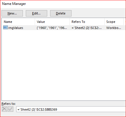
@saleemch 

Okay. Let define named range for the values as

where first row is the row with years and couple of empty rows at the end as the gap.

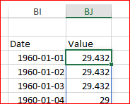
Transferred data will put here

In BF3 is the formula to calculate the date starting from the first one in our range

=DATE(INDEX(rngValues,1,1),1,ROW()-ROW($BF$2))

into BG3 we pick-up the value from the range

=IFNA(INDEX(rngValues,$BF3-DATE(YEAR($BF3),1,1)+2,MATCH(YEAR($BF3),INDEX(rngValues,1,0),0)),"out of range")

Let stay on BF3 and in reference box will enter

Entire this range will be selected. Now press Ctrl+D, formulas from BF3:BG3 will be expanded till end of this range.

Right now for leap years with have zero for 31 Dec. I didn't add any values, add them yourself where necessary.

Please check in second sheet of the attached file.

[#5]

@saleemch 

One more solution is with Power Query

- query source range

- expand it keeping dynamic list of columns

- add Index column and unpivot Years columns

- add date column based on year number and Index (aka date # within an year)

- cosmetic and load back to Excel sheet

Script is generated from UI, the only coding part is to take list of columns within the range

let
    Source = Excel.CurrentWorkbook(),
    SelectNamesRange = Table.SelectRows(Source, each [Name]="rngValues"),
    KeepContent = Table.SelectColumns(SelectNamesRange,{"Content"}),
    lstColumns = Table.ColumnNames(
        KeepContent{0}[Content]
    ),
    ExpandContent = Table.ExpandTableColumn(
        KeepContent,
        "Content",
        lstColumns,
        lstColumns
    ),
    YearsToHeaders = Table.PromoteHeaders(ExpandContent, [PromoteAllScalars=true]),
    AddIndex = Table.AddIndexColumn(YearsToHeaders, "Index", 0, 1),
    UnpivotYears = Table.UnpivotOtherColumns(AddIndex, {"Index"}, "Attribute", "Value"),
    ProperTypes = Table.TransformColumnTypes(
        UnpivotYears,
        {
            {"Attribute", Int64.Type},
            {"Value", type number}
        }
    ),
    AddDates = Table.AddColumn(
        ProperTypes,
        "Date",
        each Date.From(Date.AddDays(#datetime([Attribute],1,1,0,0,0),[Index])),
        type date
    ),
    RemoveUnused = Table.SelectColumns(AddDates,{"Date", "Value"}),
    SortByDates = Table.Sort(RemoveUnused,{{"Date", Order.Ascending}})
in
    SortByDates

Please see in the third sheet attached.

[#6]

This is my first answer to the community. Hope it does go well

I have tried to build a dynamic array which will automatically update the total no of rows as the years get increased and tried to build up the days in a single colown.

Value can be 

I have tried this formula:

=DATE(C2,1,1)+TRANSPOSE(SEQUENCE(,DAYS(DATE($BB$2,12,31),DATE($C$2,1,1))))-1

Where BB2 is 2011 and C2 is 1960.

Please refer Sheet 2 in the attachment

@Sergei Baklan 

Sir Please help.

[#7]

Thanks a lot @Sergei Baklan. It worked and solved my problem.

[#8]

@saleemch , you are welcome, glad to help

[#9]

@CA_PUNIT_AGARWAL 

If with dynamic arrays, I'd use named range instead of fixed first and last year (number of columns could be changed). When the spill

=SEQUENCE(EDATE(DATE(LARGE(INDEX(rngValues,1,0),1),1,0),12)-DATE(INDEX(rngValues,1,1),1,1),1,DATE(INDEX(rngValues,1,1),1,1),1)

and values with reference on this spill

=INDEX(rngValues,$BI$3#-DATE(YEAR($BI$3#),1,1)+2,MATCH(YEAR($BI$3#),INDEX(rngValues,1,0),0))

They are here on second sheet of the attached file.