- Subscribe to RSS Feed
- Mark Discussion as New
- Mark Discussion as Read
- Pin this Discussion for Current User
- Bookmark
- Subscribe
- Printer Friendly Page
- Mark as New
- Bookmark
- Subscribe
- Mute
- Subscribe to RSS Feed
- Permalink
- Report Inappropriate Content
Apr 26 2022 08:46 AM
I have a table with 6 columns for each month, each month alternates either blue or white. I am trying to automate the sequence so that I don't have to type it in each month. I am sure it is an easy fill/repeat thing, but it is currently escaping me. Row 2 stays the same for each month - there is no sequence there. Thank you for your help!
- Labels:
-
Excel
-
Formulas and Functions
- Mark as New
- Bookmark
- Subscribe
- Mute
- Subscribe to RSS Feed
- Permalink
- Report Inappropriate Content
Apr 26 2022 08:57 AM
Change the appearance of your worksheet
To change the text fonts, colors, or general look of objects in all worksheets of your workbook quickly, try switching to another theme or customizing a theme to meet your needs. If you like a specific theme, you can make it the default for all new workbooks.
Hope I was able to help you with this information.
I know I don't know anything (Socrates)
- Mark as New
- Bookmark
- Subscribe
- Mute
- Subscribe to RSS Feed
- Permalink
- Report Inappropriate Content
Apr 26 2022 09:11 AM
Also, I want some kind of a formula so that the first 6 columns have the heading Mar 22, the next have Apr 22, the next have May 22 and so on. I didn't think it was a theme kind of thing?
- Mark as New
- Bookmark
- Subscribe
- Mute
- Subscribe to RSS Feed
- Permalink
- Report Inappropriate Content
Apr 26 2022 10:37 AM
Solution@Edith_Thornburg , see attached file for example.
Set-up the formula as below.
Formula trend is :-
If Start is from column A, then
=DATE(2022,FLOOR((COLUMN()-1)/6,1)+3,1)If Start is from column B, then
=DATE(2022,FLOOR((COLUMN()-1-1)/6,1)+3,1)If Start is from column C, then
=DATE(2022,FLOOR((COLUMN()-1-2)/6,1)+3,1)and so on...
Once setup, you can drag the formula to the right.
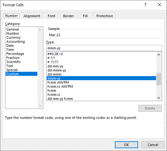
Format the cell as below setting :-
Set up 12 columns manually for color and formula.
Then select 12 columns, and drag to the right.
The formula and color shall be filled as you desire.
- Mark as New
- Bookmark
- Subscribe
- Mute
- Subscribe to RSS Feed
- Permalink
- Report Inappropriate Content
Apr 26 2022 10:55 AM
Accepted Solutions
- Mark as New
- Bookmark
- Subscribe
- Mute
- Subscribe to RSS Feed
- Permalink
- Report Inappropriate Content
Apr 26 2022 10:37 AM
Solution@Edith_Thornburg , see attached file for example.
Set-up the formula as below.
Formula trend is :-
If Start is from column A, then
=DATE(2022,FLOOR((COLUMN()-1)/6,1)+3,1)If Start is from column B, then
=DATE(2022,FLOOR((COLUMN()-1-1)/6,1)+3,1)If Start is from column C, then
=DATE(2022,FLOOR((COLUMN()-1-2)/6,1)+3,1)and so on...
Once setup, you can drag the formula to the right.
Format the cell as below setting :-
Set up 12 columns manually for color and formula.
Then select 12 columns, and drag to the right.
The formula and color shall be filled as you desire.

