Conditions formatting

[Isra_sidki]

I have two tables, and I want to compare between them, and in table 3 the results of compared show in colors how I can do this?

[#2 · Accepted solution]

@Isra_sidki 

Can you provide more explanation to the conditional format you are trying to setup? Is it the condition supposed to be less than a certain column or flag a certain text?

Also, please provide a sample workbook of how your data is structured.

[#3]

This is the attachment I want the table of tna look just in color without any text.
Thx for the responding

[#4]

@Isra_sidki 

See below how one of the TNAs are populated:

1. Assign values

I included a grading system (1-3) to make it easier for the TNA column to read the match requirements.

2. TNA Lookup Formula

=IF(OR(G14="",H14=""),"",IF(G14=H14,"MATCH",
IF(VLOOKUP(G14,Sheet1!$B$3:$C$5,2,FALSE)<VLOOKUP(H14,Sheet1!$B$3:$C$5,2,FALSE),"ABOVE","BELOW")))

This formula returns either MATCH, BELOW, or ABOVE and only populates if the Required and Current column have been populated.

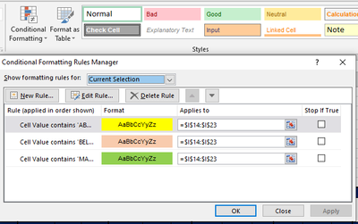
3. Conditional Format

You can modify the color scheme when managing the conditional format. There are 3 based on the text returns. The trick to having the text hidden is to have the font match the background color

You can copy and paste the TNA sample column to the others and the format and formulas will adjust.

[#5]

Thx so much I really appreciate it.