Conditional Formatting

[macsmaker]

I'm having issues understanding conditional formatting. Here's a snippet of the data:

201-015000-1
201-012410-1
STM0877-01
STM0952-0101-17925
201-012419-1
STM0878-01
STM0882-01
201-015005-1
201-015010-1
201-015110-1
201-015110-3
201-015110-5
STM0907-01
MS20426AD4-6A
MS20426AD4-7A
MS21060L5
NAS1394CA4L

I need for cells that begin with "201-" to have an orange background. I won't put all the steps for conditional formatting, the formula I'm using is 

=ISNUMBER(FIND("201-",C2,1))

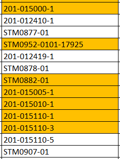
This is the result:

This is not even close. It's formatting values I DON'T want to format, for example

"STM0952-0101-17925",

but does not format items it should such as "201-012410-1."

This is TOTALLY incorrect, and very frustrating. Is there an unreported issue with Excel 0365 conditional formatting?

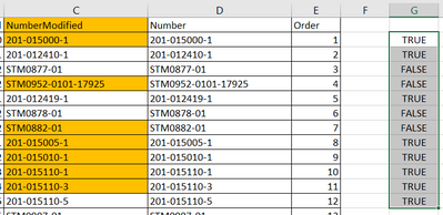
Also, if I put the formula in Column G, it finds the proper values. It's like there's an issue with how conditional formatting handles formula:

[#2]

@macsmaker 

It looks like the rule looks at the cell below the one being formatted.

When you create the rule, make sure that the active cell in the selection is the first (top) cell in the selection.

And make sure that the formula refers to that cell.

For example, if the range is C1:C17, C1 should be the active cell in the selection, and the formula should be =ISNUMBER(FIND("201-",C1,1)) or alternatively =LEFT(C1,4)="201-"

[#3]

Thanks, that fixed it. I noticed too, it was shifted, but the formula specified starting at C2, so I'm not sure why it didn't work. But, it's fixed and I can move on. Thanks so much.