Conditional formatting

[Rpm2020]

Hi Everyone, First timer here.

I am building some spreadsheets and I am having some issues with conditional formatting.

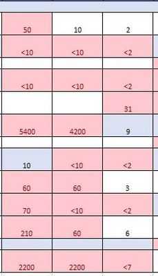
The sheet contains results from laboratory water testing and results are often reported as a number like <10. Due to testing accuracy reasons its reported as <10 rather than say 5.

With the conditional formatting I am highlighting results that are greater than a specific limit. The issue I run into is any result containing the "<" symbol will be highlighted regardless.

My question is, how do I have the conditional formatting either;

1. exclude any cell that contains the "<" symbol or

2. interpret the < as just the number (eg <10 as 10)

Keeping in mind I need to display it with the "<" symbol

In the photo below, all cells have the formatting to highlight in red any number greater than 10, all cells with the "<" symbol should not be highlighted.

 

Appreciate your assistance.

[#2]

if possible, pls share the file

[#3]

@Rpm2020 

This can be achieved by using 1 more validation set.

-> Format only cells that contain - Specific Text and beginning with - < (No double codes)

This is in addition to existing data validation on number greater than 10.

[#4]

@Rpm2020 

Assuming the first number is in the cell A2 and last number is in the cell C12, then select the range A2:C12 and make a New Rule for Conditional Formatting using the formula given below and set the format as per your choice.

=AND(ISNUMBER(A2),A2>10)

Remember to replace A2 with the first cell of whatever is your data range .

[#5]

@Rpm2020 

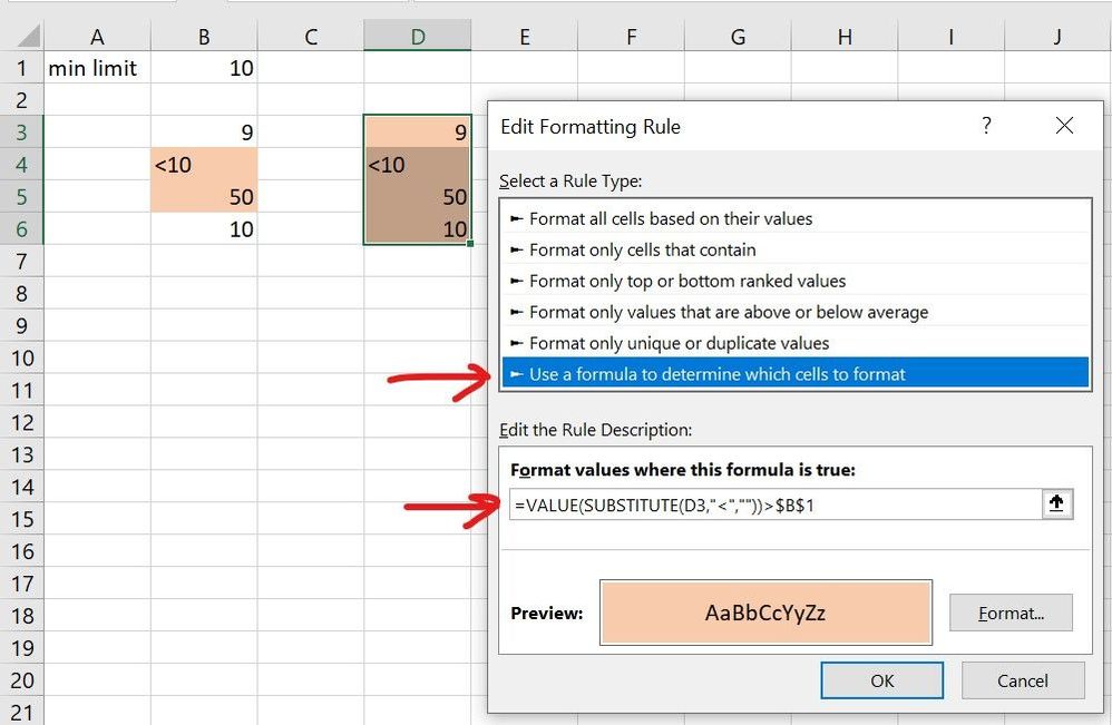
Use something like this in the conditional formula:

=VALUE(SUBSTITUTE(B3,"<",""))

Basically you're just telling xl to drop the '<'  if it's there and treat the result as a number.