- Subscribe to RSS Feed
- Mark Discussion as New
- Mark Discussion as Read
- Pin this Discussion for Current User
- Bookmark
- Subscribe
- Printer Friendly Page
- Mark as New
- Bookmark
- Subscribe
- Mute
- Subscribe to RSS Feed
- Permalink
- Report Inappropriate Content
Sep 15 2022 09:50 AM
Hi all,
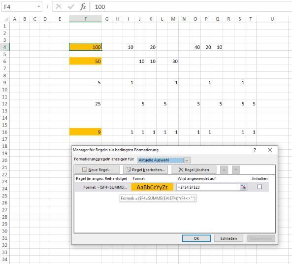
I had made a rule that turned a cell,(A4), orange once the sum of the adjacent cells,(B4:J4), were equal to the value of that cell,(A4), see image for example,
but somehow the rule has disappeared and no matter how I frame the formula it will not work.
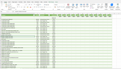
The following image is the real sheet that the rule will be used in, using the cells in column F as the target and the cells in column's I to T as the accumulators.
In English, I want the TOTAL cells in Column F to change colour when the entered value's in the adjacent DATE column's equal the total.
I really hope this makes sense.
Any help would be really appreciated.
- Labels:
-
Excel
-
Formulas and Functions
- Mark as New
- Bookmark
- Subscribe
- Mute
- Subscribe to RSS Feed
- Permalink
- Report Inappropriate Content
Sep 15 2022 10:13 AM
=($F4=SUM($I4:$T4))*(F4<>"")This rule for conditional formatting works in my sheet.
=$F$4:$F$23The "applies to" range starts in row 4 as well.


