Conditional Formatting with two columns and rows of data to 500 x 500 date set

[devesh680]

Hello Everyone,

I`m trying to create a conditional formatting excel where

1) Two columns 

    i) Being the lower end of a value <- 1st Column

   ii) Being higher end of a value<- 2nd Column

If the values in the 500 x 500 data set vary of these two particular row elements of the column then that row should be highlighted with red color.

The values in the two columns are changing row to row. 

Let me know if there is more explanation required.

Thanks

Dev

[#2]

@devesh680 

As I understood I made this file. pleas tell me if I got something wrong!

[#3]

@devesh680 

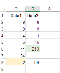
There are several methods, few I would like to show here:

How it works:

• Select Q2:R8, and hit Conditional Formatting
• Find Top & Bottom Rule, from menu hit More Rules.
• Select Format only Top or Bottom ranked values.
• Select TOP then 1 & Bottom then 1 and  apply an appropriate format, finish with Ok.

N.B. For Applied to the range, for the TOP 1 the range must be, R2:R8. and for Bottom 1 the range must Q2:Q8.

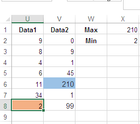
Another is the dynamic way:

• In any blank cells find Maximum & Minimum from both columns.
• Use these as rules: 

=$U2=$X$2 and =$V2=$X$1

• You may adjust cell references in the formula. 

[#4]

@devesh680 

Not everything is clear, at least for me. Looks like

- we have the range with 500 rows and 500 columns size;

- somewhere outside this range (aka data) there is another range with 500 rows and 2 columns size;

- In columns of the later are defined bounds for the correspondent rows of the data range, min in first column and max in second one

- all values in data range which are out of this bounds for the correspondent row shall be highlighted by red color

[#5]

Hello Rajesh,

In the provided example of the Excel sheet. The first two columns would be deciding factor for the rest of the dataset. I would want to highlight all the row items which wouldn't fall under this two row items of the columns.

[#6]

Hello Sergei,
You got this correct.!
In columns of the later are defined bounds for the correspondent rows of the data range, min in first column and max in second one

- all values in data range which are out of this bounds for the correspondent row shall be highlighted by red color.
This is exactly what I`m trying to do where as the bounding values for each row are varying.

[#7]

@devesh680 

That is close to what @Ramiz_Assaf  suggested. Assuming SI is column with down bound and SJ is with upper one, you may use the rule with formula

=(A1<$SI1)+(A1>$SJ1)