Conditional formatting with 3 color scale. Copy format to other cells

[JuttaWERU]

Dear experts,

How can I copy the conditional formatting of the 1st row to subsequent rows taking into account the values of the corresponding row and not the 1st one.

Thanks in advance for your support,

Jutta

[#2]

@JuttaWERU 

I am not sure I fully understand your objectives, so let's start with a simple 'solution'.

Use Format Painter to select the conditional format, then apply it to each target range separately. 

Any of the limits may be adjusted using the dialogue boxes you show, as can the colours.

[#3]

 Use conditional formatting to highlight information

Copy and paste conditional formatting

If you want to apply an existing formatting style to new or other data on your worksheet, you can use Format Painter to copy the conditional formatting to that data.

Click the cell that has the conditional formatting that you want to copy.

Click Home > Format Painter.

 

The pointer changes to a paintbrush.

Tip: You can double-click Format Painter if you want to keep using the paintbrush to paste the conditional formatting in other cells.

To paste the conditional formatting, drag the paintbrush across the cells or ranges of cells you want to format.

To stop using the paintbrush, press Esc.

Note: If you’ve used a formula in the rule that applies the conditional formatting, you might have to adjust any cell references in the formula after pasting the conditional format. For more information, see Switch between relative, absolute, and mixed references.

Hope I could help you with these information / links.

NikolinoDE
I know I don't know anything (Socrates)

@JuttaWERU

[#4]

Thanks for your proposals!

If I use the format painter, the formula always maintains the original cell reference.
But I want to have a relative reference which is not allowed in the conditional formatting.
Since the real excel has thousands of rows, I don't want to adjust the references in the formula manually.

[#5]

@JuttaWERU 

So your requirement is to create 1000s of conditional format ranges, one per row?

Rather than creating thousands of conditional formats, you might consider creating two formats each applied to the entire range.

[#6]

@JuttaWERU 

In your conditional formatting, you have absolute references.

For the sake of simplicity, you would have to convert these into relative references.
There's an old trick I use where I switch the columns in R1C1 reference type.

This makes it possible to directly use or copy/paste the conditional formatting formulas

per code Z1S1 reference type without having to switch to the settings.

After that you can remove the tick and the formulas are adjusted to their place with absolute references to the new cells.

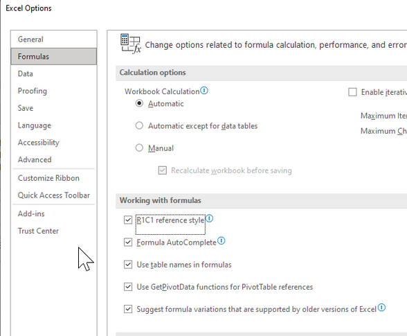
File--> Options --> Formulas --> Working with Formulas --> R1C1 Reference Style.

[#7]

@NikolinoDE 

Thank you so much for your support, but I am doing something wrong.

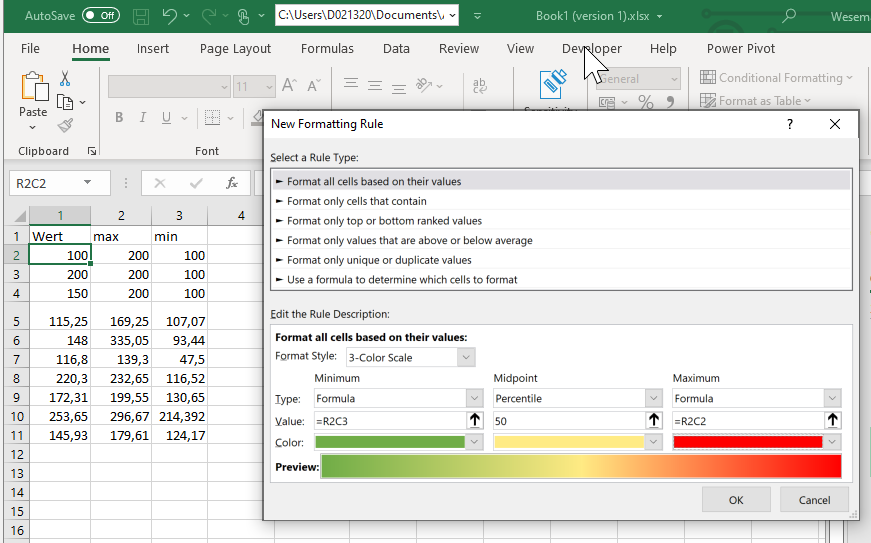
Would you be so kind having a look at the steps:

1. File--> Options --> Formulas --> Working with Formulas --> R1C1 Reference Style.

2. Conditional formatting for cell A2 considering values of C2 and D2:

3. Use Format painter to copy formula

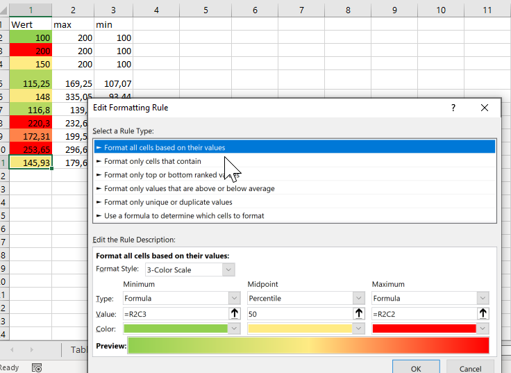
4. Check formula for row 11:

5. Remove tick in file options

6. check formula again for row 11 and there the reference is unfortunately again to row 2

@NikolinoDE, can you please show me where I am doing the mistake?

Many Thanks,+

Jutta

[#8]

@JuttaWERU 

Assume all cells have absolute references.

1. File--> Options --> Formulas --> Working with Formulas --> R1C1 Reference Style - tick the box – Ok – back to the sheet. Now they are relative reference values.
2. Select the cells/range --> Copy with Ctrl + C
3. Go to the beginning cell of the desired cell/range where to paste the copied cell/s - Ctrl + V to paste.
4. Go to File--> Options --> Formulas --> Working with Formulas --> R1C1 Reference Style - tick the box out – Ok – back to the sheet.
5. After that, all should be absolute reference values again, with the application referring to the new cells.

That's what I have in mind...if it doesn't work for you, I recommend that you send the file (without sensitive data) or as a private message (if you think you absolutely have to) to me in order to to see how the file is structured.

Otherwise you and I will have to spend far too much time, which shouldn't be the case :).

[#9]

Since I do not see when I have to do the step with the condition formatting, I sent you the excel.

[#10]

@JuttaWERU 

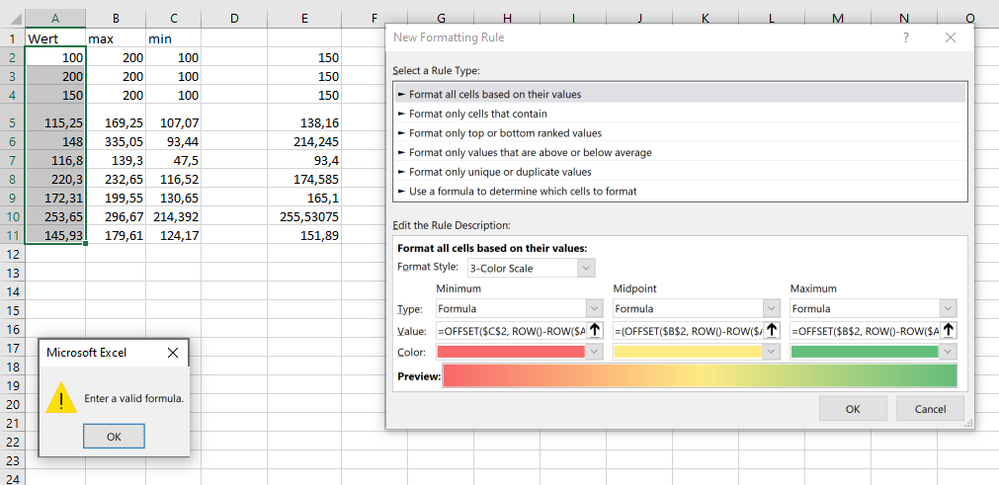
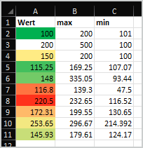
You may use OFFSET for the gradient and icons

min:
=OFFSET($C$2, ROW()-ROW($A$1)-1, 0)
midpoint:
=(OFFSET($B$2, ROW()-ROW($A$1)-1, 0)+OFFSET($C$2, ROW()-ROW($A$1)-1, 0))/2
max:
=OFFSET($B$2, ROW()-ROW($A$1)-1, 0)

[#11]

@Sergei Baklan 

Thanks for your proposal.

It works when downloading your excel , but not if I copy and past to my excel: => Invalid formula

[#12]

@JuttaWERU 

Perhaps you shall use semicolons in formula instead of commas. Could you share your file?

[#13]

I sent a message to you with the excel.

[#14]

I looked in my private message, but it's empty.

[#15]

@JuttaWERU 

Sorry didn't notice that you use a color scale.

You cannot use relative references in conditional formatted criteria for color scales, data bars, or icon sets.

You can change "Applies to" with R1C1 but no references in the reference cells.

This is only possible if you don't use color scales, data bars or icon sets in conditional formatting.

For your project, I can blindly agree with Mr. Sergei Baklan’s  proposed solution :))

Attached are Mr. Sergei Baklan’s formulas, translated into German.

Add these as instructed by Mr. Baklan.

Minimum

 =BEREICH.VERSCHIEBEN($C$2; ZEILE()-ZEILE($A$1)-1; 0)

Mittelpunkt

=(BEREICH.VERSCHIEBEN($B$2; ZEILE()-ZEILE($A$1)-1; 0)+BEREICH.VERSCHIEBEN($C$2; ZEILE()-ZEILE($A$1)-1; 0))/2

Maximum

=BEREICH.VERSCHIEBEN($B$2; ZEILE()-ZEILE($A$1)-1; 0)

Thank you for your understanding and patience

[#16]

Thanks for providing me with the German translation!
But I still have the problem that the formula refers to the 1st min and max.

[#17]

You were right, replacing the ',' by ';' did help!
But I still have the problem that also with the Offset formula min and max values are taken from B2 and C2 as absolute reference for all other values. Do you have an idea how to solve this?
Thanks,
Jutta

[#18 · Accepted solution]

@JuttaWERU 

Sorry, I  didn't test properly. It works differently compare to couple of years ago. Workaround could be

- apply the rule to $A$2 only

- using format painter apply to other cells but A3

- in CF manager duplicate rule for A2 and apply it to A3

[#19]

@Sergei Baklan 

Thank you very much for your support!

[#20]

@JuttaWERU , you are welcome