Conditional formatting traffic light system with blanks

[deemon1981]

Hi all,

I have been asked to create something and i'm really struggling to create the formula so i'm hoping someone here could help me out!

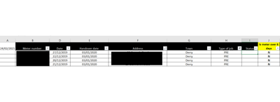
I currently have a formula in column J - =IF(E6-D6<=6,"N","Y") This tells me if a meter was handed over within our target of 6 days.

I now want to expand on this and create a traffic light visualisation so the admin staff can easily visually see what meters are almost late and can chase them up.

So in column I (status), the formula should be something like, =IF(E6-D6<=6, "GREEN IN TRAFFIC LIGHT", "RED IN TRAFFIC LIGHT").  However, if column E (handover date) is BLANK I want it to compare Column D (date) with cell A1 (todays date) and return the colours as white IF <=4 and amber IF value is between 5 and 6.  Hopefully that makes sense!

Many Thanks,

David

 

[#2]

@deemon1981 

And what if E6 is blank and D6 is more than 6 days before today's date?

[#3]

@Hans Vogelaar 

Hi,

That would mean the meter has not been handed over in time and would be red.

[#4 · Accepted solution]

@deemon1981 

Thanks. See the attached sample workbook. I created a formula in column J that returns 1, 2, 3 or 4 and used those values in the traffic light conditional formatting rule.

[#5]

@Hans Vogelaar 

Hans, you sir are a hero!  Your formula worked perfectly for me.  Thank you very much for your time and effort!  Have a great day!