Conditional formatting to highlight a cell where 2 dates match

[Jenbons]

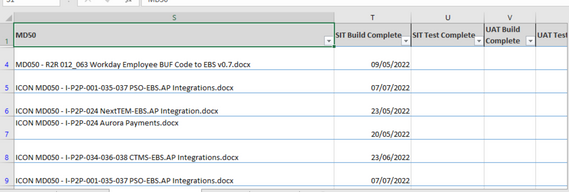
I'm trying to create a spreadsheet with a Gantt chart layout, and want to use conditional formatting to place a colour cell where a particular activity starts.  I have the dates running across the top of the Gantt on one sheet, and the project data with dates of activities in another sheet.  I'm therefore looking for a formula whereby if a date in the project data sheet matches a date running across the top of the Gantt, that cell will be coloured.  

How do I do that? 

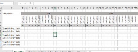
Here's the Gantt sheet: 

And this is the source project data sheet: 

[#2]

@Jenbons 

=SUMPRODUCT(($A3=Tabelle2!$C$9:$C$15)*(C$2=Tabelle2!$D$9:$D$15))

Maybe with this rule for conditional formatting.

[#3]

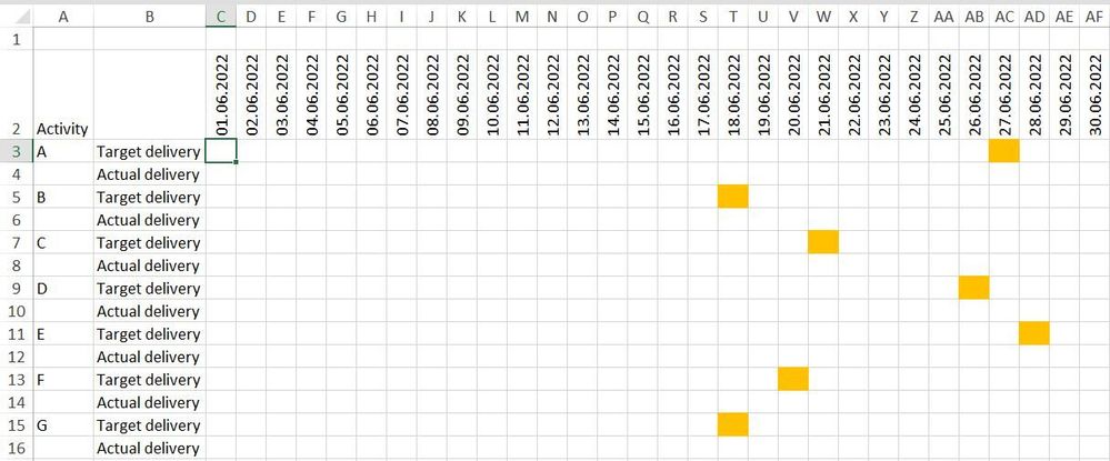
@OliverScheurich Thank you - but I can't get that to work. I've simplified things by pulling the dates into the same sheet as below - is there a simpler formula which asks if 2 dates match between row 3 and column D, shade that cell in relation to the date of row 3? 

[#4]

@Jenbons 

=$D5=G$3

You can try this rule for conditional formatting.

=$G$5:$AN$11

Above is the "Applies to" range from the attached example.

 

[#5]

Thanks so much - that's far simpler than I thought, but is working perfectly. Much appreciated!