Conditional formatting to change row color when cell value changes

[shawnc1959]

I'm trying to use conditional formatting to shade "groups" of rows when the value in column A changes (so all rows with the same value are either shaded or not).  To distinguish when the key value changes, I added a new column (N) and set the value of row 1 to be =TRUE().  Then for rows 2 thru the end, I added the formula =IF(A2=A1,N1,NOT(N1)); so effectively the value of the cell in N alternates from TRUE to FALSE when the value in A changes.  This part seems to work as intended.

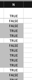
Then I created a conditional formatting rule where it adds a fill color to the row based on the formula =AND(LEN($A2)>0,$N2); so there has to be a value in column A and the value in column N must be TRUE.  It is shading some rows and not others, but not as expected; see photo:

The top row is A with =TRUE() in it, and the subsequent rows with the formula are correctly alternating between TRUE and FALSE when the key value in A is changing (effectively when the group changes).  But I can't figure out what the conditional formatting is doing.  I assume I've missed something but can't see it, so any thoughts are appreciated.

BTW, this is Excel for Mac v16.57.

[#2 · Accepted solution]

@shawnc1959 

It looks like the rule is one row off.

Delete the rule and start over.

Make sure that the active cell in the selection is in the first row of the selection.

Also make sure that the formula in the rule refers to the cell in that row in column N.

[#3]

@Hans Vogelaar It looks like the selection was off ... I was trying to apply it to all the rows in the target columns (i.e., $A:$N), but redoing it with the specific cells seemed to fix it.

Thanks!