Conditional Formatting Rule - Implicit intersection operator

[Anglex]

Hello everyone,

• Device and OS platform: win10
• Excel product name and version number: excel 365
• Excel file: excel in attached files.
• What you're trying to do - and why 
  I'm creating an excel using apache-poi.
  This excel have some parameters that has to be filled by my stakeholder.
  Some cells should highlight based on parameters on Sheet1 to help him fill the Sheet2.
  
  I had some hard time figuring out what was the issue with my formula but I guess that it has to with implicit intersection operator .
  
  In my code I'm adding this string as in a cell and as a conditional formatting rule:
  

"ISNUMBER(FIND(\"|#|\"&XLOOKUP(INDIRECT(\"'Sheet2'!\"&ADDRESS(1,COLUMN()))&INDIRECT(\"'Sheet2'!\"&ADDRESS(2,COLUMN())),Sheet1!$1:$1&Sheet1!$2:$2,Sheet1!$3:$3,\"NotFound\")&\"|#|\", \"|#|a|#|b|#|c|#|d|#|\"))"

however when I saw it in excel cell it gave me this result:

=ISNUMBER(FIND("|#|"&@XLOOKUP(@INDIRECT("'Sheet2'!"&ADDRESS(1,COLUMN()))&@INDIRECT("'Sheet2'!"&ADDRESS(2,COLUMN())),@Sheet1!$1:$1&@Sheet1!$2:$2,Sheet1!$3:$3,"NotFound")&"|#|", "|#|a|#|b|#|c|#|d|#|"))

As you can see some '@' were inserted.
Then when I click enter on the formula, a pop-up ask me if I want to use this variation instead:


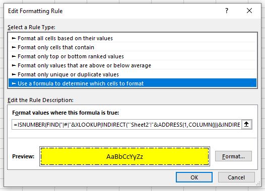
In conditional formatting rule, this modification seems implicit.
That means when I go to my rule, look at it and click 'ok'. Excel fix the formula somehow.
It doesn't show any additional '@' either:

I really can't ask all my stakeholder to fix it manually.

• Expected result and method to achieve the result**
  
  Highlight the cells as expected using the required parameters.
  A method to avoid this additional '@'.
  
  

Thank for your knowledge,
Best regard
Alex

[#2 · Accepted solution]

@Anglex 

Excel has two calculation methods, implicit intersection and dynamic array. Historically, excel used implicit intersection by default for worksheet formulas, but dynamic array by default for other things like conditional formatting and names. 

More here: https://exceljet.net/glossary/implicit-intersection

With Office 365, MS changed the worksheet formula default calculation method to dynamic array. The implicit intersection operator "@" can be used to force excel to use implicit intersection (more commonly, you probably see it used more in structured table references). 

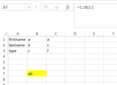
With your formula, for example, the part where you are concatenating rows 1:1&2:2, this is what implicit intersection returns (screenshot) - it will only return the result corresponding to the same column as the formula (since I entered the formula in column B, it concatentates B1&B2). If I want Excel to return all of the results in versions prior to office 365, I need to force dynamic array by hitting Ctrl+Shift+Enter after keying the formula.

I think you probably want the formula calculated as an array in 365 and prior versions. If you are setting the formula via code, then you may want to further research the Formula, Formula2, and FormulaArray properties of the range object to confirm which one you want (I believe with office 365, you want Formula2 for dynamic array, Formula is implicit intersection - this may be why it's showing up in your worksheet with the "@" symbol). I'm not sure if you would want formula2 or formulaarray for backwards compatibility (if that's an issue, have to research or test it further).

But, if backwards compatibility is an issue, you can't use xlookup. So, you'll probably need to use Iferror(Index(Match())) (which appears to work okay on my machine):

B3=ISNUMBER(FIND("|#|"&IFERROR(INDEX(Sheet1!3:3,MATCH(INDIRECT("'Sheet2'!"&ADDRESS(1,COLUMN()))&INDIRECT("'Sheet2'!"&ADDRESS(2,COLUMN())),Sheet1!1:1&Sheet1!2:2,0)),"Not Found")&"|#|", "|#|a|#|b|#|c|#|d|#|"))

[#3]

Hello,

Thank for your answer, I will definitively test and research what you mention.

Best regard,

[#4]

@Anglex 

UDFs or built in functions like INDIRECT tend to cause Excel problems when compatibility with legacy spreadsheet paradigm is required because it can't tell whether such functions will return an array or a scalar value.  Excel tends to sprinkle '@'s like confetti, just to make sure.  Personally, I would prefer to move away from constructs like ADDRESS and INDIRECT and use defined names to identify data, e.g.

= ISNUMBER(FIND("\"&XLOOKUP(fName&lName, firstname&lastname, type)&"\", "\a\b\c\d\"))

as an array formula or define 'CFormat?' to generate the single cell relative references that are required to make the antiquated conditional formatting work correctly

= ISNUMBER(FIND("\"&XLOOKUP(@fName&@lName, firstname&lastname, type)&"\", "\a\b\c\d\"))