- Home
- Microsoft 365
- Excel
- Re: Conditional Formatting over different sheets in a workbook
Conditional Formatting over different sheets in a workbook
- Subscribe to RSS Feed
- Mark Discussion as New
- Mark Discussion as Read
- Pin this Discussion for Current User
- Bookmark
- Subscribe
- Printer Friendly Page
- Mark as New
- Bookmark
- Subscribe
- Mute
- Subscribe to RSS Feed
- Permalink
- Report Inappropriate Content
Jul 12 2020 05:07 AM
Hello
I use a workbook with 9 Different sheets,
Each sheet is for a different case.
For Example: The workbook is for our products,
Sheet1 = Orders which are completed
Sheet2 = Orders ready for billing
Sheet3 = Orders with technical issues
sheet4 = Orders with mechanical/replacement Issues
and so on..,
Every sheet has few columns but in all the sheets, there are 3 columns which are common,
A: Order Number B: Location C: Date
What i want to establish is, If Order 5674 is entered in column A of "Ready for Billing " sheet and if i mistakenly entered the same order number in Column A of "Technical Issues" it should color the cell in RED saying its a Duplicate.
( I cannot use any kind of 3rd party tools or software but i want to achieve this using conditional formatting or writing a module)
Thank you Upfront for your time. Your Ideas are greatly appreciated. :)
- Labels:
-
Formulas and Functions
- Mark as New
- Bookmark
- Subscribe
- Mute
- Subscribe to RSS Feed
- Permalink
- Report Inappropriate Content
Jul 12 2020 07:56 AM - edited Jul 12 2020 09:54 AM
I created two sheets:
1. Ready for billing
2. Technical issues
On each sheet, I created a Named Table (use Ctrl+T or Home>Format as Table) with three columns:
1. Order number
2. Location
3. Date
The tables are named (respectively):
1. readyforbilling
2. technicalissues
I place my cell in the first row of the technicalissues table in the Order number column, then I create a rule using Home>Conditional Formatting>New Rule, where I select "Use a formula to determine which cells to format".
The formula used in the rule is:
=NOT(ISERROR(VLOOKUP($A3,'Ready for billing'!$A:$A,1,FALSE)))
When I am editing the second parameter of the VLOOKUP formula, I click the column header of the first column (A) on the Ready for Billing sheet, such that it selects the entire column.
As you likely know, a conditional formatting formula must return either TRUE or FALSE.
This formula is looking for the order number from the current row in the technicalissues table in the order number column of the readyforbilling table. If it's found, VLOOKUP will return the order number from column 1 of the readyforbilling table, and so will not be an error. As such, the entire formula will return TRUE (because NOT inverts the return value of ISERROR, which would be FALSE).
If the order number is not found, VLOOKUP will return an error, ISERROR will return TRUE and NOT(ISERROR will return FALSE.
The net effect is that order numbers found in the readyforbilling table are formatted and those which are not, are not.
Because we are using Tables, the Applies To range will expand as each new row is added.
- Mark as New
- Bookmark
- Subscribe
- Mute
- Subscribe to RSS Feed
- Permalink
- Report Inappropriate Content
Jul 12 2020 08:17 AM
Thankyou so much for your efforts. Really appreciate it.
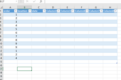
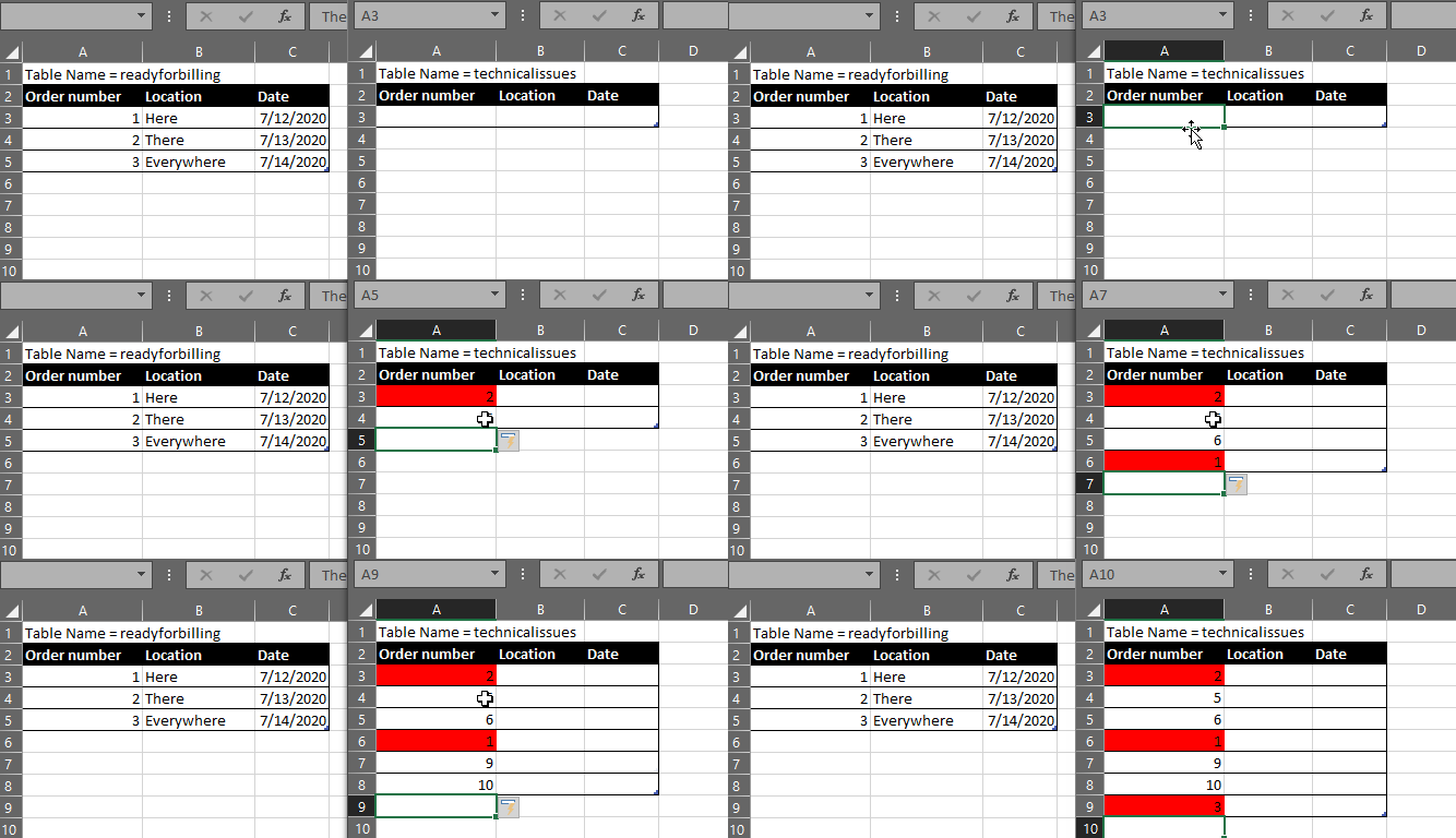
I exactly did what you have done ( Applied formula in order column, for Tech Issues sheet) and still, this is what i am seeing. Am i doing some thing wrong?
- Mark as New
- Bookmark
- Subscribe
- Mute
- Subscribe to RSS Feed
- Permalink
- Report Inappropriate Content
Jul 12 2020 09:21 AM
- Mark as New
- Bookmark
- Subscribe
- Mute
- Subscribe to RSS Feed
- Permalink
- Report Inappropriate Content
Jul 12 2020 09:33 AM
- Mark as New
- Bookmark
- Subscribe
- Mute
- Subscribe to RSS Feed
- Permalink
- Report Inappropriate Content
Jul 12 2020 09:52 AM
Solution
Ok, since you are starting with data in the table, please go to the Conditional Formatting Rules Manager using Home>Conditional Formatting>Manage Rules.
Then, click the arrow to edit the Applies To range:
Now put your cursor above the "order" column until you see a black arrow. When you see the black arrow, left-click so that the whole column is selected:
Then click the down-arrow on the Conditional Formatting Rules Manager shown above.
Now select the rule and click Edit Rule.
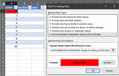
Select the part of the formula that says $A3 and then click on the first row in the technicalissues table. For you, this will be changing it to $A2:
When you first click the cell, it will show $A$2. You need to remove the second $. You can do this by deleting it, or by pressing F4 twice to cycle through relative and absolute references.
Next, highlight the part of the formula that gives the range to the Ready for Billing sheet:
While that is highlighted, go to the Ready for Billing sheet and again, select the entirety of column A by clicking on the A column header:
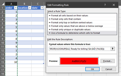
In the end, your rule formula will look something like this:
=NOT(ISERROR(VLOOKUP($A2,'Ready for billing'!$A:$A,1,FALSE)))
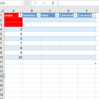
Now that you have deliberately selected the entire column for the lookup range, and repositioned your starting cell, you should have no problems with newly added rows.
- Mark as New
- Bookmark
- Subscribe
- Mute
- Subscribe to RSS Feed
- Permalink
- Report Inappropriate Content
Jul 12 2020 12:57 PM
Thankyou so much @OwenPrice
This worked perfect and i am able to apply the same formula vice versa on all sheets.
Thankyou for your time and efforts.
Have a great day.
Accepted Solutions
- Mark as New
- Bookmark
- Subscribe
- Mute
- Subscribe to RSS Feed
- Permalink
- Report Inappropriate Content
Jul 12 2020 09:52 AM
Solution
Ok, since you are starting with data in the table, please go to the Conditional Formatting Rules Manager using Home>Conditional Formatting>Manage Rules.
Then, click the arrow to edit the Applies To range:
Now put your cursor above the "order" column until you see a black arrow. When you see the black arrow, left-click so that the whole column is selected:
Then click the down-arrow on the Conditional Formatting Rules Manager shown above.
Now select the rule and click Edit Rule.
Select the part of the formula that says $A3 and then click on the first row in the technicalissues table. For you, this will be changing it to $A2:
When you first click the cell, it will show $A$2. You need to remove the second $. You can do this by deleting it, or by pressing F4 twice to cycle through relative and absolute references.
Next, highlight the part of the formula that gives the range to the Ready for Billing sheet:
While that is highlighted, go to the Ready for Billing sheet and again, select the entirety of column A by clicking on the A column header:
In the end, your rule formula will look something like this:
=NOT(ISERROR(VLOOKUP($A2,'Ready for billing'!$A:$A,1,FALSE)))
Now that you have deliberately selected the entire column for the lookup range, and repositioned your starting cell, you should have no problems with newly added rows.

