Conditional Formatting on Concatenate Formula

[milo1234]

Hi Team, I have successfully created a conditional formatting concatenate formula, however when the columns are copied and new ones are inserted, the conditional formatting cells are using the old columns and not basing them on the new columns.

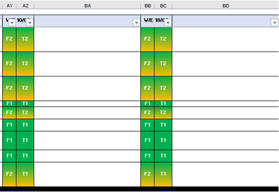
For example: I copy columns AY and AZ into BB and BC, however the formula is picking up AY and AZ still.

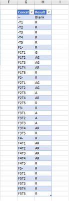
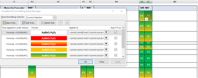
I have attempted to resolve this issue numerous times, however I have had no luck. Please find print screens attached. 

=VLOOKUP(CONCATENATE($BB3,$BC3),Legend!$G$2:$H$38,2,FALSE)="Blank"

=VLOOKUP(CONCATENATE($BB3,$BC3),Legend!$G$2:$H$38,2,FALSE)="R"

=VLOOKUP(CONCATENATE($BB3,$BC3),Legend!$G$2:$H$38,2,FALSE)="AR"

=VLOOKUP(CONCATENATE($BB3,$BC3),Legend!$G$2:$H$38,2,FALSE)="A"

=VLOOKUP(CONCATENATE($BB3,$BC3),Legend!$G$2:$H$38,2,FALSE)="AG"

=VLOOKUP(CONCATENATE($BB3,$BC3),Legend!$G$2:$H$38,2,FALSE)="G"

[#2]

Hi, I'm a little confused about the issue. You say, "I copy columns AY and AZ into BB and BC, however the formula is picking up AY and AZ still." but then the formula you give is "=VLOOKUP(CONCATENATE($BB3,$BC3),Legend!$G$2:$H$38,2,FALSE)="Blank""
That said, I think you problem is the $ in the Concatenate formula. On one hand you are using it to force both columns to concatenate the correct cells but then when you copy to new columns it is preventing it from looking at and acting on the new columns.
IF you have blank columns to the left and right of each set as you show above you could make the formula:
=VLOOKUP(CONCATENATE(BA3:BC3),Legend!$G$2:$H$38,2,FALSE)="Blank"

So in this solution cell BB3 would apply the above formula and concatenate BA3:BC3 which would be blank & BB3 & BC3 and give what you want. Then BC3 would concatenate the offset/relative cells BB3:BD3, but again assuming those blank columns would be BB3 & BC3 & blank and again give you what you want. Of course this ONLY works if there are blank columns on both sides.
There are other tricks you can play if you know that the columns of interest are always a fixed amount apart (e.g. columns 10,11 and 20,21 and 30,31 ....) and then you can use the column value to offset the cell and make sure it concatenates the correct set. So in the below formula if the column is divisible by 10 then concatenate (I just use the & operator) the next cell but if not then use the previous cell:
=VLOOKUP(BB3&OFFSET(BB3,0,IF(MOD(COLUMN(BB3),10),-1,1)),Legend!$G$2:$H$38,2,FALSE)="Blank"

Another trick could be to use the column header to do the offset. For example it looks like the column header of the 1st column in each pair is "W/E". so the following might work:
=VLOOKUP(BB3&OFFSET(BB3,0,IF(BB$1="W/E",1,-1)),Legend!$G$2:$H$38,2,FALSE)="Blank"

I hope that helps

[#3]

@mtarler Thank you for your suggestions, however they have not resolved the issue. 

The formula I provided showed cells AY and AZ, as I amended this formula, however they originally showed BB and BC when copied and inserted. 

The columns either side will not be blank, these are always filled with text however I removed this as they contained sensitive data. 

I have attached sample data - please could you have a go and see if you can resolve? 

Thank you for your help. 

[#4]

@milo1234 I created 1 conditional formatting formula you can use as a template:

=VLOOKUP(IFS(LEFT(I$2,3)="W/E",I1&J1,LEFT(H$2,3)="W/E",H1&I1,1,""),Legend!$B$2:$C$38,2,FALSE)="AG"

This was applied to the entire region I:BD and should work as long as the pair of columns you want it applied to are the only columns that start with "W/E".

[#5]

@mtarler Thank you for this. I have applied the formula to all relevant columns with the correct colour coding. It seems to work for most of the cells, however in the sample data attached, if I change a cell to F1 and T1 this should be green together, however one cell shows (F1) as green and the other cell as red (T1). 

Also when I copy the 3 columns and insert these copied cells for a new week, the cells that the conditional formatting applies to, changes. 

Please can you help? 

[#6 · Accepted solution]

@milo1234  there was a typo in one of the formulas that references row E instead of H.  I fixed that so I hope the attached works for you.

As for copy and paste, yes it will "change" the applied to and the formula but that should be ok.  What it is doing is COPYING both the applied to range and formula and shifting the cell references according to the new location.  You can see that if under conditional formatting you use the drop-down at the top and set it to "This Worksheet" and you will see 'duplicate rules'.  And after a bit of copy, paste, insert, and such that conditional formatting drives my OCD crazy and I have to 'clean it up' but that is cosmetic and not functional issues. 

[#7]

@mtarler Thank you again, this is really useful. 

I can see you resolved the formula, however when you copy columns BH, BI & BJ for a new week and insert the copied cells, the same issue applies. 

T1 and F1 does not change to green together - what can I do to stop this? 

[#8]

the easiest is to not "insert copied cells", just PASTE. If you need to insert columns then do that 1st then copy and paste. That is interesting what "insert copied cells" does, not sure if that is a bug or not and might be useful trick in certain cases.

[#9]

@mtarler Thank you so much for helping, I really appreciate it :)