Conditional Formatting not working with text

[Danimal513]

on one tab I have a list of names

on a second tab I have a list of the names and next to them in another cell an A, B, or C ranking

I want the first tab to match the name in the second tab to the ranking next to it and color the cell based on the latter ranking.

This works if the names are numbers, but once it is actual text names it doesn't work properly. I am making this in a google sheets doc as I do not have 365 to do filter formulas.

Using this coding:

=VLOOKUP(E2,indirect("Names!B2:C115"),2,TRUE) = "A"

In the pictures the rankings are the same. A(green) for 1-29 B(Yellow) 30-70 C(Red)71-114. All names are from a name generator and not actual names. Just trying to make the function work properly.

Thank you,

Dan

[#2]

Since you've created a spreadsheet with false names, why don't you post it, rather than just posting an image. That way you wouldn't be forcing us to create our own copy....we could work with your anonymous data.

[#3 · Accepted solution]

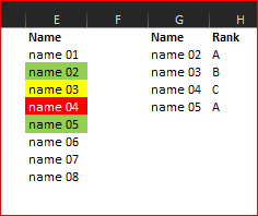
@Danimal513 

Here is working sample

Conditional formatting rule formulae as

=INDEX($H$2:$H$5,MATCH(E2,$G$2:$G$5,0)) = "A"

[#4]

Thank you so much! Since it was in google sheet I had to modify it slightly to;
=INDEX(indirect("Hires!$C$2:$C$115"),MATCH(E2,indirect("Hires!$B$2:$B$115"),0)) = "A"
being on a different tab. Super helpful, and much appreciated!!!

[#5]

@Danimal513 , you are welcome