- Home
- Microsoft 365
- Excel
- Conditional formatting in a column that highlights the cell if it matches data in another worksheet
Conditional formatting in a column that highlights the cell if it matches data in another worksheet
- Subscribe to RSS Feed
- Mark Discussion as New
- Mark Discussion as Read
- Pin this Discussion for Current User
- Bookmark
- Subscribe
- Printer Friendly Page
- Mark as New
- Bookmark
- Subscribe
- Mute
- Subscribe to RSS Feed
- Permalink
- Report Inappropriate Content
Aug 14 2022 06:16 PM - edited Aug 14 2022 08:05 PM
Hello!
I am wanting to apply a conditional format formula that will highlight a cell in a colmun if it contains the same data from a column in another sheet. The formula I have found is not working and just highlights the entire colmun when I apply it. The formula I have found is the following formula: =NOT(ISERROR(VLOOKUP($B3,'Sheet2'!A:A,1,FALSE)))
- Labels:
-
Formulas and Functions
- Mark as New
- Bookmark
- Subscribe
- Mute
- Subscribe to RSS Feed
- Permalink
- Report Inappropriate Content
Aug 14 2022 07:53 PM
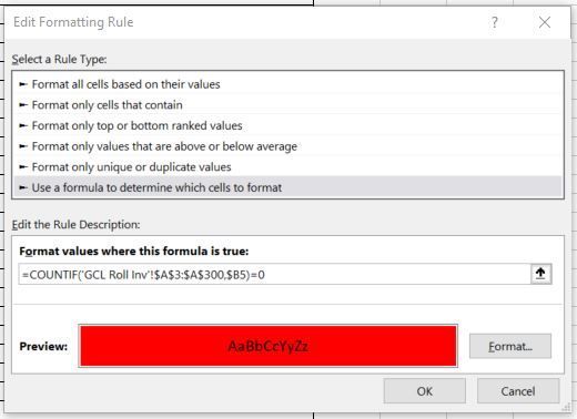
@Catherine_Robertshawe try using this in the conditional formatting menu.
=Countif('sheet 1'!$C$2:$C$5,$B2)=0
That seemed to work for me. You will need to put a second rule in so that it doesn't highlight the blanks though.
- Mark as New
- Bookmark
- Subscribe
- Mute
- Subscribe to RSS Feed
- Permalink
- Report Inappropriate Content
Aug 14 2022 08:09 PM
- Mark as New
- Bookmark
- Subscribe
- Mute
- Subscribe to RSS Feed
- Permalink
- Report Inappropriate Content
Aug 14 2022 09:20 PM
@Catherine_Robertshawe I just realised that the formula that I gave you will highlight everything that isn't the same. If you replace the =0 with =1 it should work.
This is what I've got in mine to highlight any cells that don't match the column/range on the other sheet.
